Tutorial on Statistical Computing for Extremes with R
Bayesian inference
2023-06-30
Bayesian inference
- Combine likelihood with a prior: posterior.
\[ p(\boldsymbol{\theta} \mid \boldsymbol{Y}) = \frac{p(\boldsymbol{Y} \mid \boldsymbol{\theta})p(\boldsymbol{\theta})}{ \int p(\boldsymbol{Y} \mid \boldsymbol{\theta})p(\boldsymbol{\theta})\mathrm{d}\boldsymbol{\theta}}, \qquad(1)\]
- Posterior is proper (if likelihood times prior is integrable).
- Parameters asymptotically normal in large samples under general conditions.
- Need to evaluate integral in denominator (normalizing constant that does not depend on \(\boldsymbol{\theta}\)).
Change of paradigm
In the Bayesian world,
- inference is conditional on observations,
- parameters are treated as random variables
- (reflecting uncertainty about their true value).
Inference
In all scenarios, we will have samples from the posterior distribution for parameters \(\boldsymbol{\theta}\): any summary can be computed from these via Monte Carlo methods.
e.g., we can report the posterior mean or median
credible intervals (probability that parameter falls in) are simply quantiles of functionals
Prediction
We consider new realizations from posterior predictive \[\begin{align*} p(Y_{\text{new}} \mid \boldsymbol{Y}) = \int_{\Theta} p(Y_{\text{new}} \mid \boldsymbol{\theta}) p(\boldsymbol{\theta} \mid \boldsymbol{Y}) \mathrm{d} \boldsymbol{\theta} \end{align*}\]
- For every posterior draw \(\boldsymbol{\theta}_b\) \((b=1, \ldots, B)\), sample new realization from generative model.
- Marginalization means discarding \(\boldsymbol{\theta}_b\)’s
Why bother?
- Priors can act as penalty
- regularizing parameter estimates in small samples.
- Natural extensions via hierarchical modelling (e.g., random effects).
- Expert knowledge can be encoded through the priors.
Intractable models
Trade optimization for integration problem!
The integral is intractable, so we need to resort to alternative schemes:
- Numerical integration via Laplace approximations (INLA)
- Monte Carlo methods to simulate (approximate) draws from the posterior
Monte Carlo methods
- Most packages implement offer Markov chain Monte Carlo algorithms
- gives approximate correlated draws
- requires tuning
- need to check convergence
For models without covariates, Northrop (2023) offers exact draws from posterior via the ratio-of-uniform algorithm.
Bayesian dispute
One objection to Bayesian inference is arbitrary selection of priors
- Influence of the prior vanishes as sample size grows unless it imposes support constraints!
- Likelihood are also often used for convenience
- Same for lasso and ridge (\(L_1\) and \(L_2\)) penalties in regression.
Prior selection
- Typically, parameters are assumed independent apriori (so prior factorizes), even if posterior doesn’t
- Choosing proper priors (density functions) ensure proper posteriors.
- Care is needed, especially for shape parameter
Priors for extreme value models (1/2)
Popular choices include
- improper uniform priors
- vague or diffuse Gaussian priors, e.g., \(\xi \sim \mathsf{No}(0, 10)\)
- Jeffrey’s prior (invariant to reparametrization.
- for generalized Pareto \[\sigma^{-1}(1+\xi)^{-1}(1+2\xi)^{-1/2}\mathrm{I}_{\xi > -1/2}\]
- invalid for the GEV regardless of sample size(Northrop & Attalides, 2016)!
Priors for extreme value models (2/2)
Better choices penalize the shape, including
- Martins & Stedinger (2001) prior \(\xi + 0.5 \sim \mathsf{Beta}(6, 9)\)
- Maximal data information (MDI): \(\sigma^{-1}\exp\{-a(1+\xi)\}\mathrm{I}_{\xi \geq -1}\) Northrop & Attalides (2016)
- Prior on quantiles (Coles & Tawn, 1996), back-transformed
Impact of priors
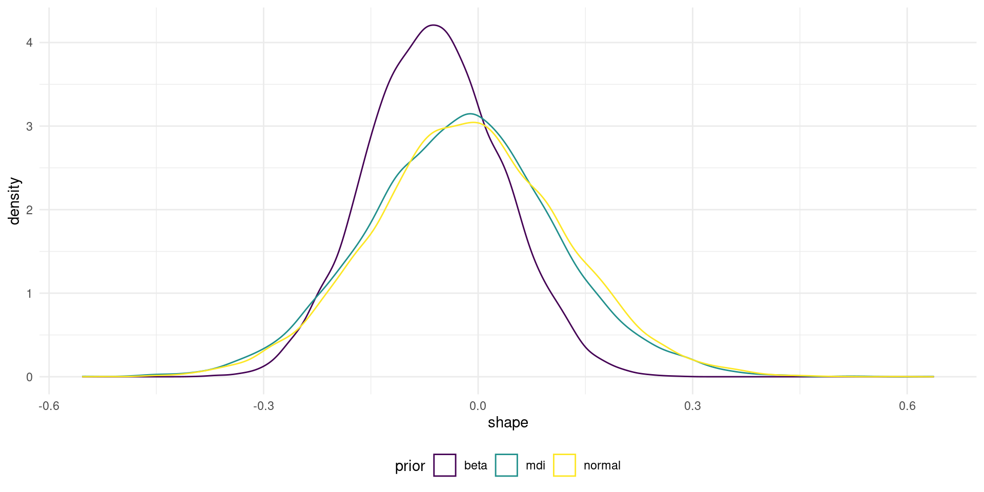
Figure 1: Marginal posterior of GEV shape parameter for different prior distributions.
Ratio-of-uniform sampling
The revdbayes (Northrop, 2023) provides the state-of-the-art for stationary models (faster than MCMC, exact sampling).
Point estimators and credible intervals
For each combination of posterior draw, compute the functional of interest (e.g., the median of the 50-year maximum) and/or quantiles.
Posterior predictive samples
Here, using max-stability to get a new observation (maximum of 50 yearly max) for each draw \(\boldsymbol{\theta}\).
Posterior predictive
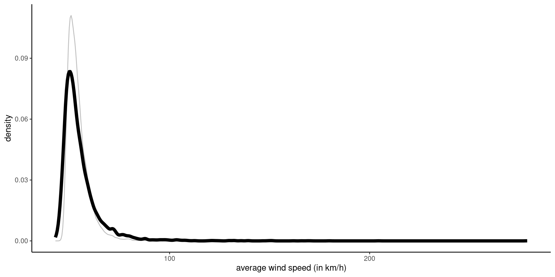
Figure 2: Density of posterior predictive (black) and posterior median (grey) of 50 year maximum.
Diagnostics for Bayesian workflow
Can model capture summaries of data?

See bayesplot and loo packages for more information and options about the Bayesian workflow (Gabry et al., 2019).
Regression model
Posterior estimates
Family:       GEV

Posterior summary:
                 Posterior mean        SD
mu: (Intercept)     36.30933484 0.7041629
mu: syear           -0.66354673 0.7182214
phi: (Intercept)     1.44282072 0.1293479
xi: (Intercept) -0.04462734 0.1352223Monitoring Markov chain Monte Carlo
- run multiple Markov chains from different starting values
- discard initial samples (burn-in)
- check convergence:
- are all chains converging to the same region
- are chains stationary?
Effective sample size
With multiple chains, it is easier to use output of coda package.
For summaries to be reliable (e.g., quantiles of posterior), the approximate number of independent samples from the total simulated should be large enough.
chains <- coda::as.mcmc.list(
  lapply(post_reg$chains, coda::as.mcmc))
# effective sample size is sufficient here
coda::effectiveSize(chains)
var1 var2 var3 var4
2763.133 3121.967 3024.125 3093.349 Can compare algorithms efficiency via effective sample size per second.
Traceplots
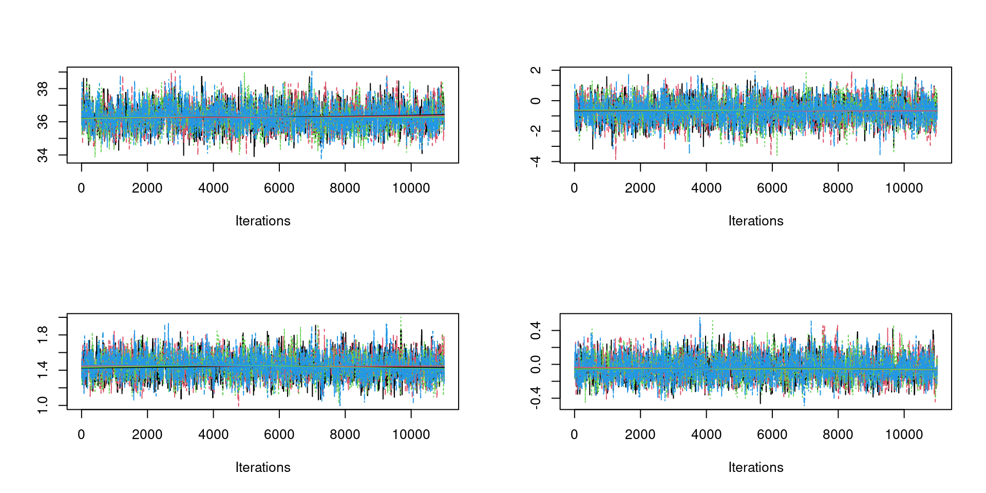
Should look like fat hairy catterpilars.
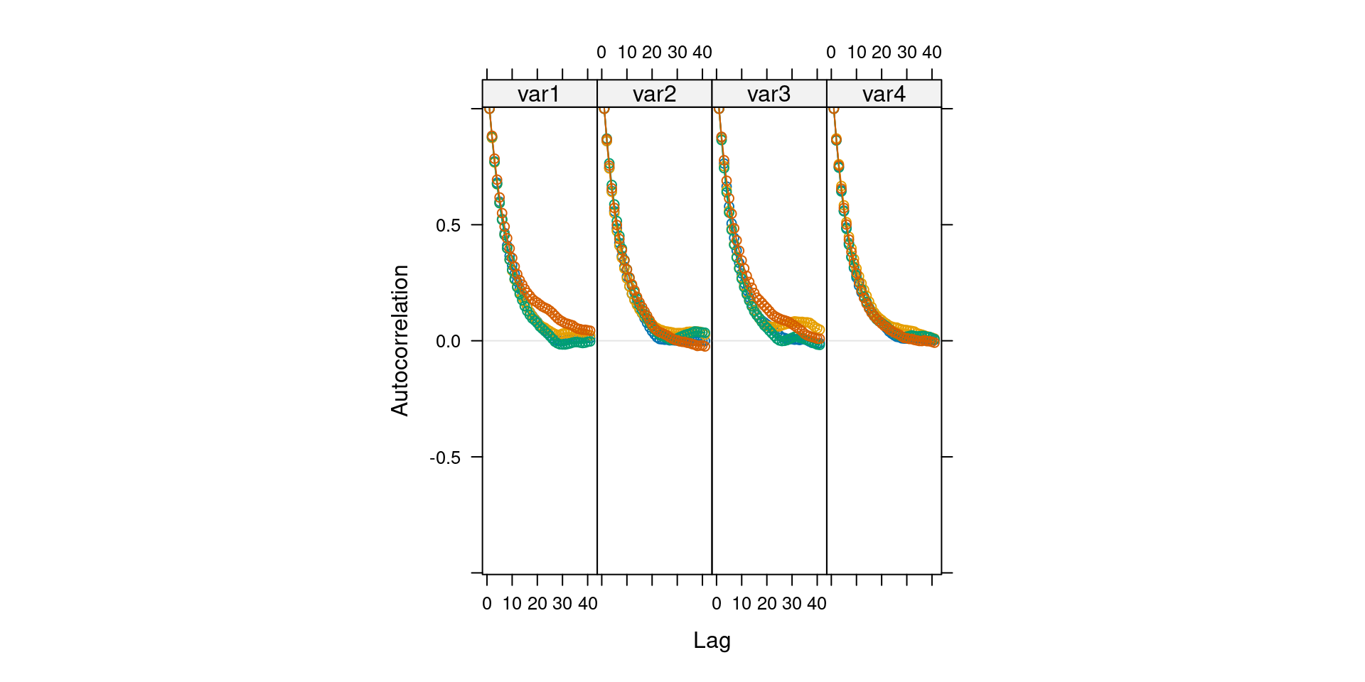
Algorithm efficiency
While some MCMC algorithms are more costly, they yield samples that are less autocorrelated (so contain more information altogether).
- Is autocorrelation reasonable?
- Related to acceptance rate (Goldilock principle)
- Ideally, algorithms sample parameters on unconstrained space
- Good proposals adapt to the local geometry and satisfy support constraints
Correlograms
Summaries
We can get directly summaries (e.g., posterior sample mean)
- standard errors for functionals is more complicated due to the autocorrelation
Due to autocorrelation, dedicated methods are employed to get standard errors.
       V1              V2                V3              V4
 Min.   :33.91   Min.   :-3.1841   Min.   :1.064   Min.   :-0.46361
 1st Qu.:35.81   1st Qu.:-1.1247   1st Qu.:1.352   1st Qu.:-0.13404
 Median :36.30   Median :-0.6561   Median :1.436   Median :-0.05592
 Mean   :36.31   Mean   :-0.6523   Mean   :1.441   Mean   :-0.04522
 3rd Qu.:36.78   3rd Qu.:-0.1614   3rd Qu.:1.525   3rd Qu.: 0.04187
 Max.   :38.73   Max.   : 1.7285   Max.   :1.910   Max.   : 0.41994
Loss function
Custom loss function for the return levels \(q\) from EVA data challenge \[\begin{align*} L(q, \widehat{q}(\theta)) = \begin{cases} 0.9(0.99q - \widehat{q}), & 0.99q > \widehat{q} \\ 0, & |q - \widehat{q}| \leq 0.01 q\\ 0.1(\widehat{q} - 1.01q), & 1.01q < \widehat{q}. \end{cases} \end{align*}\]
Bayesian evaluation of loss function
For given value of the return level \(q_0\): \[\begin{align*} r(q_0) = \int_{\boldsymbol{\Theta}}L(q(\boldsymbol{\theta}), q_0) p (\boldsymbol{\theta} \mid \boldsymbol{y}) \mathrm{d} \boldsymbol{\theta} \end{align*}\] and we seek to minimize the risk, \(\mathrm{min}_{q_0 \in \mathbb{R}_{+}} r(q_0)\)
Loss function
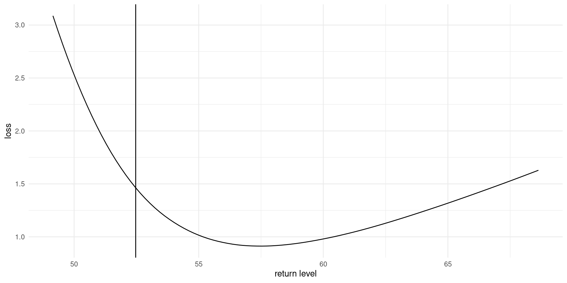
Figure 3: Loss function for wind speed data, based on fitting a generalized extreme value distribution to annual maxima.
References
revdbayes: Ratio-of-uniforms sampling for Bayesian extreme value analysis.