Tutorial on Statistical Computing on Extremes with R - Tutorial on Statistical Computing for Extremes with R

Basics of likelihoods

Denote by \(\boldsymbol{\theta} \in \mathcal{S} \subseteq \mathbb{R}^p\) the parameter vector.
Assume data has joint density \(f(\boldsymbol{y}; \boldsymbol{\theta})\).
The log likelihood is \(\ell(\boldsymbol{\theta}) = \log f(\boldsymbol{y}; \boldsymbol{\theta})\).
If the \(n\) observations are independent with density or mass function \(f_i\), then \(\ell(\boldsymbol{\theta}) = \sum_{i=1}^n \log f_i(y_i; \boldsymbol{\theta})\).
The maximum likelihood estimate \(\widehat{\boldsymbol{\theta}}\) is found by maximizing (numerically) \(\ell(\boldsymbol{\theta})\).

Why use maximum likelihood?

Easy to generalize to complex settings (nonstationarity, regression models, censoring, rounding, etc.)
Known to be asymptotically most efficient (Cramér–Rao bound), even if they can be biased in small samples.
Point estimators, etc. are invariant to reparametrization.

Extremal type theorem

Consider \(Y_i\) \((i=1,2,\ldots)\) i.i.d. with distribution \(F\).

If there exist normalizing sequences \(a_n>0\) and \(b_n \in \mathbb{R}\) such that \[\begin{align} \lim_{n \to \infty} \Pr\left(\frac{\max_{i=1}^n Y_i - b_n}{a_n} \leq x \right) = G(x), \label{eq:gevconv} \end{align}\] for \(G\) a non-degenerate distribution, then \(G\) must be generalized extreme value (GEV).

Generalized extreme value distribution

With location \(\mu \in \mathbb{R}\), scale \(\sigma \in \mathbb{R}_{+}\) and shape \(\xi \in \mathbb{R}\) parameters, the distribution function is \[\begin{align*} G(x) =\begin{cases} \exp\left\{-\left(1+\xi \frac{x-\mu}{\sigma}\right)^{-1/\xi}_{+}\right\}, & \xi \neq 0;\\ \exp\left\{-\exp\left(-\frac{x-\mu}{\sigma}\right)\right\}, & \xi = 0, \end{cases} \end{align*}\] where \(x_{+} = \max\{x, 0\}\).

The support is \(\{x \in \mathbb{R}: \xi(x-\mu)/\sigma > -1\}\).

Max-stability property

If \(Y_i \sim \mathsf{GEV}(\mu, \sigma, \xi)\) are independent, then \[\max_{i=1}^N Y_i \sim \mathsf{GEV}(\mu_N, \sigma_N, \xi),\] where

\(\mu_N = \mu + \sigma(N^\xi-1)/\xi\)
\(\sigma_N = \sigma N^\xi\)

(case \(\xi=0\) defined by continuity).

Block maximum

We can

partition data into blocks of roughly equal size \(m\) and
fit a GEV distribution to the maximum of the blocks.

library(mev)
library(xts)
library(lubridate)
data(frwinds, package = "mev")
lyon <- with(frwind, 
             xts(x = S2, order.by = date))
# Create series of yearly maximum
ymax <- apply.yearly(lyon, max)

Fitting GEV using `mev` package

opt_gev <- mev::fit.gev(xdat = ymax, show = TRUE)
## Log-likelihood: -142 
## 
## Estimates
##     loc    scale    shape  
## 36.1845   3.9429  -0.0112  
## 
## Standard Errors
##   loc  scale  shape  
## 0.659  0.488  0.132  
## 
## Optimization Information
##   Convergence: successful 
##   Function Evaluations: 30 
##   Gradient Evaluations: 14
mle <- coef(opt_gev)

Goodness-of-fit diagnostics

Custom methods (print, plot, coef, etc.) are defined

methods(class = "mev_gev")
## [1] anova  coef   logLik nobs   plot   print  vcov  
## see '?methods' for accessing help and source code
par(mfrow = c(1,2))
plot(opt_gev)

Numerical tricks

Standardize observations (e.g., scale) to facilitate optimization — the GEV is a location-scale family.
Even if the limit is continuous and well defined at \(\xi=0\), the log likelihood and it’s derivatives involves terms of the form \(\log(1+\xi x)\), which are numerically unstable when \(\xi \to 0\).
- Pro tip: do not code the likelihood yourself! Otherwise,
  - use high precision arithmetic, e.g., log1p
  - replace the terms that blow up by Taylor series expansion near \(\xi=0\) (interpolation).

Score vector

When the log likelihood is differentiable, the MLE is the root of the score equation, meaning \(\ell_{\boldsymbol{\theta}}(\widehat{\boldsymbol{\theta}}) = \left.\partial \ell(\boldsymbol{\theta}) / \partial \boldsymbol{\theta} \right|_{\boldsymbol{\theta} = \widehat{\boldsymbol{\theta}}} = \boldsymbol{0}_p\).

mev::gev.score(par = mle, dat = ymax) # score
## [1]  4.44e-08 -5.53e-08 -1.49e-07

Gradient-based algorithms exploit this feature for optimization
but beware of support constraints!

Best to reparametrize so that the parameter space is \(\mathbb{R}^p\) if possible.

Information matrix and standard errors

We can extract standard errors by taking the square root of the diagonal elements of the inverse of either

the Fisher information, \(\imath(\boldsymbol{\theta}) = \mathsf{Cov}\{\ell_{\boldsymbol{\theta}}(\boldsymbol{\theta})\}\) or
the observed information \(\jmath(\boldsymbol{\theta}) = - \partial^2 \ell(\boldsymbol{\theta})/ \partial \boldsymbol{\theta} \partial \boldsymbol{\theta}^\top\),

both evaluated at the MLE \(\widehat{\boldsymbol{\theta}}\).

# Compute observed information matrix
jmat <- mev::gev.infomat(par = mle, dat = ymax)
# Compute standard errors
sqrt(diag(solve(jmat)))
##   loc scale shape 
## 0.659 0.488 0.132
# Compare with opt$std.err

Some remarks

We may compute \(j(\widehat{\boldsymbol{\theta}})\) (the negative Hessian of log likelihood) numerically through finite differences.

Many software implementations compute MLE via Nelder–Mead simplex algorithm:

check the gradient and/or
the log likelihood differences

to make sure the optimisation was successful.

Properties of MLE

Maximum likelihood estimators are asymptotically Gaussian whenever \(\xi > -1/2\) with data in domain of attraction of extreme value distribution.
Consistency requires that one increases block size, etc. as \(n\) increases at a particular rate depending on \(F\).

Regularity conditions

Some cumulants (moments of derivatives of the log likelihood) of extreme value models do not exist.

the MLE does not solve the score equation if \(\widehat{\xi} \leq -1\)
MLE is not unique for \(\xi < -1\) (some combinations of \(\mu\) and \(\sigma\) yield infinite log likelihood).
- restrict the parameter space to \(\{\boldsymbol{\theta}: y_1, \ldots, y_n \in \mathrm{supp}(\boldsymbol{\theta}), \xi \geq -1\}\)
- For GEV, MLE at boundary is \((\widehat{\mu}=\overline{y}, \widehat{\sigma} = \max(y) - \overline{y}, \xi=-1)\).

Regularity conditions

If \(\widehat{\xi} < -1/2\), cannot evaluate the information matrix.

Regularity assumptions do not apply! reported std. errors are misleading.
Typically faster convergence, joint limit not asymptotically normal (Smith, 1985).

In applications, shape is typically close to zero, so authors sometimes restrict \(\xi \in (-0.5, 0.5)\).

Penalization of the shape helps ensure that we get reasonable estimates in small samples.

Invariance property of maximum likelihood

If \(h\) is a mapping, then \(h(\widehat{\boldsymbol{\theta}})\) is the MLE of \(h(\boldsymbol{\theta})\).

The expected value of the \(N=50\)-years maximum for \(\xi < 1\), is \[\begin{align*}\mathfrak{e}_N = h(\mu, \sigma, \xi) = \mu_N + \sigma_N\{\Gamma(1-\xi)-1\}/\xi. \end{align*}\]

Thus, the MLE \(\widehat{\mathfrak{e}}_N=h(\widehat{\mu}, \widehat{\sigma}, \widehat{\xi})\).

# MLE of expectation of maximum of 50 blocks
gev.mle(xdat = ymax, args = "Nmean", N = 50)
## Nmean 
##  53.4

Profile log likelihood

Consider a functional of interest \(\psi\) and other parameters \(\boldsymbol{\lambda}\), treated as nuisance.

We reparametrize the log likelihood in terms of \((\psi, \boldsymbol{\lambda})\) and compute the profile log likelihood \[\begin{align*} \ell_{\mathrm{p}}(\psi) = \max_{\boldsymbol{\lambda}} \ell(\psi, \boldsymbol{\lambda}) \end{align*}\]

Plot of profile

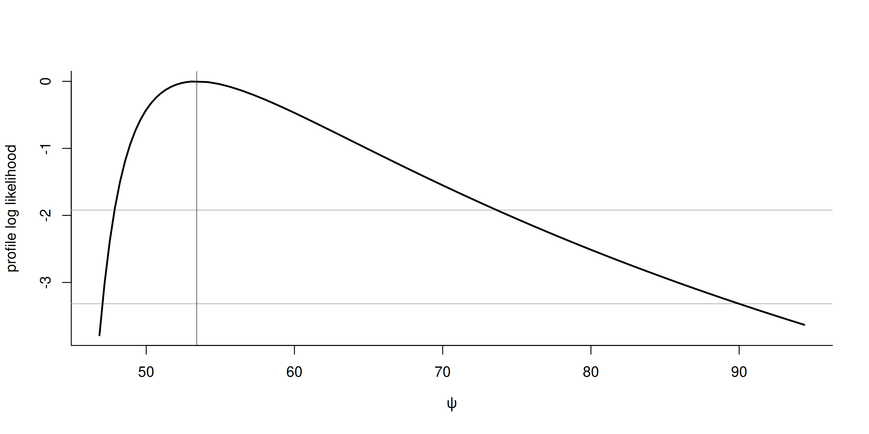
prof <- mev::gev.pll(param = "Nmean", dat = ymax, N = 50)

Confidence intervals

Under regularity conditions, the likelihood ratio statistic \[\begin{align*} 2 \{\ell_{\mathrm{p}}(\widehat{\psi}) - \ell_{\mathrm{p}}(\psi_0)\} \stackrel{\cdot}{\sim} \chi^2_1 \end{align*}\] For the hypothesis \(\psi = \psi_0\), a \((1-\alpha)\) confidence interval based on the profile likelihood ratio test is \[\begin{align*} \{\psi: 2\{\ell(\hat{\theta}) - \ell(\hat{\theta}_{\psi})\} \leq \chi^2_1(1-\alpha)\}. \end{align*}\]

(confint(prof))
## Estimate Lower CI Upper CI 
##     53.4     47.9     73.6

Generalized Pareto

If extremal type theorem applies, then threshold exceedances \(Y-u \mid Y>u\) follow, as \(u\) tends to the upper endpoint of \(F\), a generalized Pareto distribution.

The generalized Pareto distribution is \[\begin{align*} H(y; \tau, \xi) &= \begin{cases} 1-\left(1+\xi {y}/{\tau}\right)_{+}^{-1/\xi}, & \xi \neq 0,\\ 1- \exp \left(-{y}/{\tau}\right)_{+},& \xi = 0, \end{cases} \label{eq:gpdist} \end{align*}\]

Preprocess data

Choose a threshold \(u\) (either an order statistic or a fixed quantity) and extract exceedances
Use Grimshaw (1993) algorithm to reduce the 2D optimization problem to a line search.

windlyon <- with(frwind, S2[month(date) <= 4 | month(date) >= 9])
qulev <- 1-100/nrow(windlyon)
u <- quantile(windlyon, 1-100/length(windlyon))

Fitting the generalized Pareto model

opt_gp <- mev::fit.gpd(
  xdat = windlyon, threshold = u, show = TRUE)
## Method: Grimshaw 
## Log-likelihood: -208 
## 
## Threshold: 33.8 
## Number Above: 90 
## Proportion Above: 0.008 
## 
## Estimates
##  scale   shape  
## 3.5786  0.0309  
## 
## Standard Errors
## scale  shape  
## 0.609  0.134  
## 
## Optimization Information
##   Convergence: successful

Modelling bulk

The generalized Pareto only describes what happens above the threshold, but we can use the empirical distribution below: \[\begin{align*} \widehat{\Pr}(Y_i \le x) = \sum_{i=1}^n \mathsf{I}(Y_i \le x)/n, \qquad x \leq u. \end{align*}\]

Many splicing models propose a (semi)parametric model for the bulk; see evmix package for examples

Binomial - generalized Pareto model

The binomial-generalized Pareto model includes a likelihood contribution for \(\mathsf{I}(Y_i >u) \sim \mathsf{Bin}(1, \zeta_u)\), where \(\zeta_u = \Pr(Y_i >u)\).
This third parameter is orthogonal to the others, and there is a closed-form solution for the MLE.

Block maximum vs threshold exceedances

Suppose we fit a \(\mathsf{GP}(\tau, \xi)\) distribution to exceedances above \(u\).
If there are on average \(N_y\) observations per year, the distribution of the \(N\)-year maximum conditional on exceeding \(u\) is approximately \(H^{\zeta_uNN_y}\).

Threshold stability

Mathematical basis for extrapolation.

If \[\begin{align*} Y - u \mid Y>u \sim \mathsf{GP}(\tau, \xi), \end{align*}\] then for \(\{v >u\in \mathbb{R}_{+}: \tau+\xi (u-v)>0\}\),
\[\begin{align*} Y-v \mid Y>v \sim \mathsf{GP}\{\tau + \xi (u-v), \xi\}, \end{align*}\] and \(\zeta_v = \{1+\xi(v-u)/\tau\}^{-1/\xi}\zeta_u\).

Threshold stability plots

Assuming data are exactly generalized Pareto, expect shape parameters to be constant (up to sampling variability).

useq <- quantile(windlyon, seq(0.9, 0.99, by = 0.01))
tstab.gpd(windlyon, 
          method = "profile",
          thresh = useq)

Threshold stability for shape

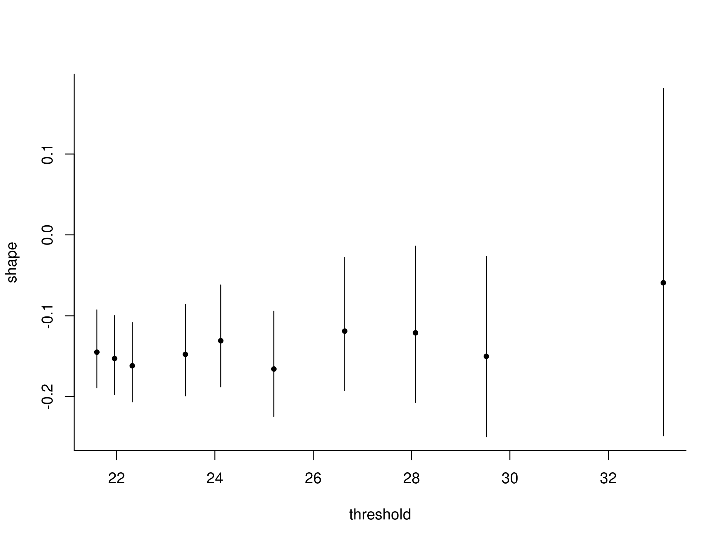
Figure 1: Threshold stability plot for Lyon mean wind speed

Inhomogeneous point process

Let \(Y_i\) i.i.d. from \(F\) with lower endpoint \(x^*\).

Consider \(a_n>0\) and \(b_n \in \mathbb{R}\) such that the distribution of the bidimensional point process \[\begin{align*} P_n =\left\{ \frac{i}{n}, \frac{Y_i-b_n}{a_n}, i = 1, \ldots, n\right\} \end{align*}\] converges to an inhomogeneous Poisson point process on sets of the form \((a, b) \times (z, \infty)\) for \(0 \leq a \leq b \leq 1\) and \(z>z_*=\lim_{n \to \infty} \{(x_*-b_n)/a_n\}\).

Intensity of inhomogeneous Poisson process

The intensity measure of the limiting point process, which gives the expected number of points falling in a set is \[\begin{align*} &\Lambda\{(a, b) \times (z, \infty)\} \\&\quad = (b-a)\left(1+ \xi \frac{z-\mu}{\sigma}\right)_{+}^{-1/\xi} \label{eq:pp_conv} \end{align*}\] for \(\xi \neq 0\).

Likelihood of the point process

\[\begin{align*} \mathcal{L}(\boldsymbol{\theta}; \boldsymbol{y}) &= (c\sigma)^{n_u} \prod_{i=1}^{n_u} \left(1+\xi\frac{y_i-\mu}{\sigma}\right)^{-1-1/\xi}_{+} \\& \times \exp\left\{- c \left(1+ \xi \frac{u-\mu}{\sigma}\right)^{-1/\xi}_{+}\right\}, \end{align*}\] The constant \(c\) is introduced as a way to relate the parameters of the point process likelihood to those of the GEV fitted to blocks of size \(m\) observations, e.g., \(c=n/m\).

Moins et al. (2023) propose a orthogonal reparametrization.

Link between parametrizations

Under the Poisson approximation to the binomial, the expected number of observations above the threshold is \[\begin{align*} c \left\{1+ \xi \left( \frac{u-\mu}{\sigma}\right)\right\}^{-1/\xi} \approx n_u. \end{align*}\] We can thus relate \(\mathsf{GP}(\tau, \xi)\) with Poisson, where MLE is \[\begin{align*} \mu_0 & \approx u - \sigma_0\{(n_u/c)^{-\widehat{\xi}}-1\}/\widehat{\xi}, \\\sigma_0 &\approx \widehat{\sigma}_u (n_u/c)^{\widehat{\xi}}, \qquad \xi_0 = \widehat{\xi}. \end{align*}\]

u <- quantile(windlyon, 0.99)
opt.pp <- fit.pp(
  xdat = windlyon, 
  threshold = u, 
  show = TRUE,
  np = diff(range(lubridate::year(frwind$date))))
## Log-likelihood: -267 
## 
## Threshold: 33.1 
## Number Above: 104 
## Proportion Above: 0.009 
## Number of periods: 47 
## 
## Estimates
##     loc    scale    shape  
## 36.3327   3.9506  -0.0592  
## 
## Standard Errors
##   loc  scale  shape  
## 0.537  0.380  0.107  
## 
## Optimization Information
##   Convergence: successful 
##   Function Evaluations: 8 
##   Gradient Evaluations: 5

Return levels

The probability \(p_l\) that a \(N\)-year return level is exceeded \(l\) times in \(N\) years of independent annual maxima is \(\mathsf{Bin}(N, 1/N)\).
For large \(N\), a Poisson approximation yields \(p_0=p_1=0.368\), \(p_2=0.184\), \(p_3=0.061\), etc.
- The probability of at least one exceedance over \(N\) years is in fact roughly \(0.63\).
- The return level corresponds to the 0.368 quantile of the \(N\)-year maximum distribution.

References

Grimshaw, S. D. (1993). Computing maximum likelihood estimates for the generalized Pareto distribution. Technometrics, 35(2), 185–191. https://doi.org/10.1080/00401706.1993.10485040

Moins, T., Arbel, J., Girard, S., & Dutfoy, A. (2023). Reparameterization of extreme value framework for improved Bayesian workflow. Computational Statistics & Data Analysis, to appear. https://doi.org/https://doi.org/10.1016/j.csda.2023.107807

Smith, R. L. (1985). Maximum likelihood estimation in a class of nonregular cases. Biometrika, 72(1), 67–90. https://doi.org/10.1093/biomet/72.1.67