Tutorial on Statistical Computing for Extremes with R
Regression models for nonstationary extremes
2023-06-30
Nonstationarity
There are various forms of nonstationarity, including
- trends,
- time-varying variance,
- seasonality,
- covariate effects.
No general theory
Solution 1: preprocessing
- detrend data to approximate stationary.
- for financial time series, fit ARMA-GARCH model
- use Box-Cox transformation with regression model
- analyze residuals \(R_i = Y_i - \widehat{f}(\mathbf{X}_i)\), where the postulated model is such that \(\mathsf{E}(Y_i) = f(\mathbf{X}_i)\).
Benefit: more data are available to estimate trends.
Estimating probability of rare events
\[\begin{align*} &\Pr(Y_i > y \mid \mathbf{X}_i) \\\quad &= \Pr\{R_i > y - \widehat{f}(\mathbf{X}_i)\mid \mathbf{X}_i\} \\\quad & = \Pr\{R_i > y - \widehat{f}(\mathbf{X}_i)\mid \mathbf{X}_i, R_i > u\}\Pr(R_i > u) \\& \qquad + \Pr\{R_i > y - \widehat{f}(\mathbf{X}_i)\mid \mathbf{X}_i, R_i\leq u\}\Pr(R_i \leq u) \end{align*}\] where the first term of the last line can be estimated using a generalized Pareto and the latter empirically.
Solution 2: hierarchical models
We can also incorporate parameters in the parameters of the extreme value distribution.
- Model \(g_{\mu}(\mu; \mathbf{X})=f_{\mu}(\mathbf{X}; \boldsymbol{\beta}_{\mu})\), \(g_{\sigma}(\sigma; \mathbf{X})=f_{\sigma}(\mathbf{X}; \boldsymbol{\beta}_{\sigma})\)
- Link functions \(g\), functions of covariates \(f\)
- Typically keep shape constant.
For explanatories \(\mathbf{X}\), fit regression models of the form \[\begin{align*} f(\mathbf{X}) = \beta_0 + \beta_1 \mathrm{X}_1 + \cdots \beta_p \mathrm{X}_p, \end{align*}\] and estimate parameters by maximum likelihood.
Generalized additive models
Rather than linear effects or changepoints (if \(\mathrm{X}_j\) is binary), we could consider smooths
\[\begin{align*} f(\mathrm{X}_j) = \sum_{k=1}^K \beta_k b_k(\mathrm{X}_j) \end{align*}\] where \(b_k\) are (compactly-supported) basis functions.
Scale input first! More numerically stable.
Parsimony is key
- There are few exceedances or extremes…
- The support restriction translates into up to \(n\) inequality constraints: difficult to optimize.
Take home message: keep models simple!
Penalized regression
Penalization to enforce sparsity or regularize estimation.
- For generalized additive models (GAM), penalize square of second derivative to control the wiggliness of the function.
- Smooth matrix \(\mathbf{S}\) with entries \(S_{ij} = \int b_i''(x) b_j''(x)\mathrm{d} x\), so the penalty is \(\lambda \boldsymbol{\beta}^\top \mathbf{S}\boldsymbol{\beta}\) for \(\lambda > 0\).
- These correspond to improper (i.e., rank-deficient) Gaussian priors.
Tuning parameter
Maximization over \[\begin{align*} \max_{\lambda \in \mathbb{R}_K^{+}} \max_{\boldsymbol{\beta}} \left\{\ell_{\boldsymbol{\lambda}}(\boldsymbol{\beta}) - \frac{1}{2} \boldsymbol{\beta}^\top\mathbf{S}_{\boldsymbol{\lambda}}\boldsymbol{\beta}\right\} \end{align*}\] where \(\mathbf{S}_{\boldsymbol{\lambda}} = \sum_{k=1}^K \lambda_k \mathbf{S}_k\).
- Optimal value of \(\boldsymbol{\lambda}\) obtained by maximizing the marginal likelihood, integrating out \(\boldsymbol{\beta}\) using Laplace’s method (Wood et al., 2016).
A word of caution
- With time-varying covariates, we need forecasts to compute risk measures in future.
- Model often fitted only at specific covariate values (careful at extrapolation beyond range).
- Rather than linear trend in time, use covariates that incorporate said trends but are more natural (e.g., climate model output).
Return levels under nonstationarity
In nonstationary models, risk measures of interest are defined conditionally on the value of covariates
For example, the \(1-p\) conditional return level is (Eastoe & Tawn, 2009) \[\begin{align*} \Pr(Y_t > y \mid \mathbf{X}_t =\boldsymbol{x}_t) = p \end{align*}\]
Unconditional return levels
These can be obtained by averaging out over the distribution of covariates that are employed in the model.
\[\begin{align*} \Pr(Y_t > y)=\int_{\mathcal{X}} \Pr(Y_t > y \mid \mathbf{X}_t =\boldsymbol{x}_t) \mathrm{d} P(\boldsymbol{x}_t)=p. \end{align*}\]
May require information about future distribution of covariates if these are time-varying.
As such, return levels may be meaningless quantities.
Threshold stability
The generalized Pareto model with varying scale and shape is not threshold-stable unless, for any \(v>u\), \[\begin{align*} \sigma_v(\boldsymbol{x}_t) = \sigma_u(\boldsymbol{x}_t) + (v-u) \xi(\boldsymbol{x}_t) \end{align*}\]
Restrictive! For constant \(\xi\), need \(\sigma\) linear or constant (log scale) (Eastoe & Tawn, 2009).
Using the inhomogeneous Poisson point process representation avoids these problems.
For nonstationary threshold models \(u(\mathbf{X})\), see Section 3.2.2 of Northrop & Jonathan (2011).
Software
Function evgam from the eponymous package (Youngman, 2022) builds on the mgcv package (Wood, 2017).
The setup is evgam(formula, data, family, ...), where
familyis the character string for the extreme value distribution (gev,gpd,rlargandaldfor asymmetric Laplace, used in quantile regression),formulais a list of formula for parameters (in the order location, scale, shape).
Formulas and smooth
Use s for smooths and te for tensor products of smooths (interactions)
kcontrols the number of breakpointsbscontrols the basis function, e.g., thin-plate splines (tp), cubic regression splines (cr), cyclic cubic spline (cc).fx: control whether fixed degrees of freedom for regression spline or else penalized regression spline (default,FALSE)
Data setup
Example with evgam
evgam output
** Parametric terms **

location
            Estimate Std. Error t value Pr(>|t|)
(Intercept)    36.55       0.67   54.63   <2e-16

logscale
            Estimate Std. Error t value Pr(>|t|)
(Intercept)     1.36       0.12   10.96   <2e-16

shape
            Estimate Std. Error t value Pr(>|t|)
(Intercept)    -0.12       0.14   -0.88     0.19

** Smooth terms **

location
         edf max.df Chi.sq Pr(>|t|)
s(year) 2.34      9   5.22    0.101
Fitted splines
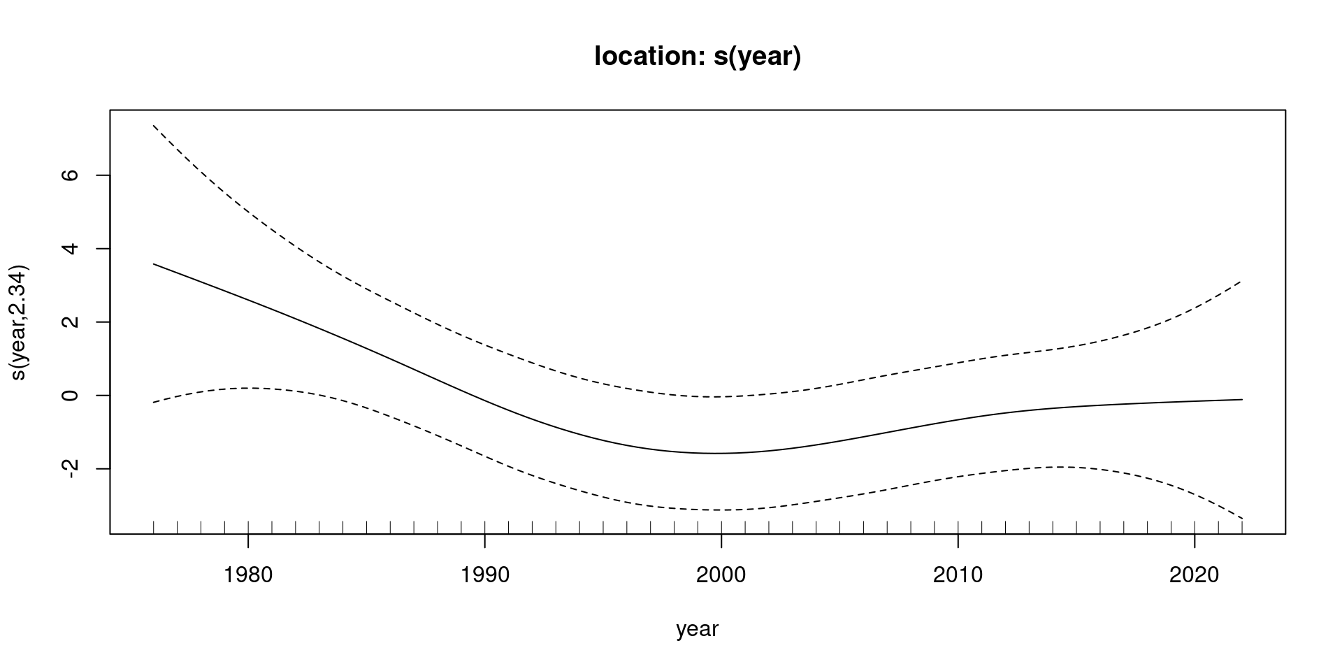
Figure 1: Fitted spline for location parameter of generalized extreme value distribution as a function of day of year (scaled to unit interval).
Plot and generalized analysis of deviance suggests constant location.
Estimated quantiles
For given \(p\), solve nonlinear equation \[\prod_{i=1}^n F^N(z; \boldsymbol{\theta}_i, \mathbf{X}_i) = p\] using qev to give unconditional quantile.
Return levels (direct method)
[1] 49.14449These return levels are meaningless, since time increases (but would lead to extrapolate beyond range of observed time)…
Quantile regression
We can work the asymmetric Laplace distribution to build a working likelihood for quantile regression at probability level \(\tau\).
The latter has density function \[\begin{align*} f(y; \mu, \sigma) = \frac{\tau(1-\tau)}{\sigma} \exp\left\{-\rho_\tau \left(\frac{y-\mu}{\sigma}\right)\right\}, \end{align*}\] where \(\rho_\tau(y) = y(\tau-\mathrm{I}_{y <0})\) is the check function.
Time-varying threshold with quantile regression
Temporal trend

Extract exceedances
Return levels
References
evgam: An R package for generalized additive extreme value models. Journal of Statistical Software, 103(1), 1–26. https://doi.org/10.18637/jss.v103.i03