Lecture 3

Upworthy archive

library(patchwork)
library(ggplot2)
theme_set(theme_classic())
suppressPackageStartupMessages(library(brms, warn.conflicts = FALSE))
library(priorsense)
data(upworthy_question, package = "hecbayes")
# Moment matching - posterior parameters
alpha <- 0.25
beta <- 25
summary_stats <- upworthy_question |>
  dplyr::group_by(question) |>
  dplyr::summarize(
    total_impressions = sum(impressions),
    total_clicks = sum(clicks)) |>
  dplyr::ungroup() |>
  as.vector()
n_yes <- summary_stats$total_impressions[1]
y_yes <- summary_stats$total_clicks[1]
n_no <-  summary_stats$total_impressions[2]
y_no <- summary_stats$total_clicks[2]
set.seed(1234)
post_data_upworthy_question <- 
  data.frame( 
  yes = rgamma(n = 1e4, shape = alpha + y_yes, rate = beta + n_yes),
  no = rgamma(n = 1e4,  shape = alpha + y_no, rate = beta + n_no))
# Posterior mean of risk ratio
post_mean <- with(post_data_upworthy_question, mean(no/yes))

We could also use brms interface to Stan to fit the Poisson regression model. The parameter here by default is on the log scale and is set on the difference between groups, but we remove the intercept so that both parameter have the same prior. Since we are taking a Gaussian prior for the log rate, we can consider a log-Gaussian distribution, and taking a mean of \(\log(0.01)=-4.6\) with a standard deviation of \(1\) gives more or less reasonable proportions. The parameters are sampled using Markov chain Monte Carlo (more later in the trimester), but the output consists of posterior samples.

headline_mod <- brm(
  clicks ~ offset(log(impressions)) + 0 + question, 
  family = poisson(link = "log"),
  data = upworthy_question,
  prior = set_prior(
    prior = "normal(-4.60517, 1)",  
    # log(0.01) = -4.60517
    class = "b"),
  backend = "cmdstanr",
  silent = 2
  )
# Summary for model coefficients
fixef(headline_mod, probs = c(0.25,0.75))

             Estimate   Est.Error      Q25      Q75
questionyes -4.512663 0.001702493 -4.51384 -4.51151
questionno  -4.441961 0.001159441 -4.44274 -4.44118

post_samp <- brms::posterior_samples(
  headline_mod, 
  pars = c("questionno","questionyes"))

ggplot() +
 geom_density(
    data = post_samp,
    mapping = aes(x = (b_questionyes - b_questionno)),
    alpha = 0.5, 
    col = 4) +
  geom_density(
    data = post_data_upworthy_question,
    mapping = aes(x = log(yes)-log(no)),
    alpha = 0.5, 
    linetype = "dashed",
    col = 2) +
  labs(x = "log of rate difference", y = "",
       caption = expression(log(lambda["yes"]) - log(lambda["no"]))) +
  theme_classic()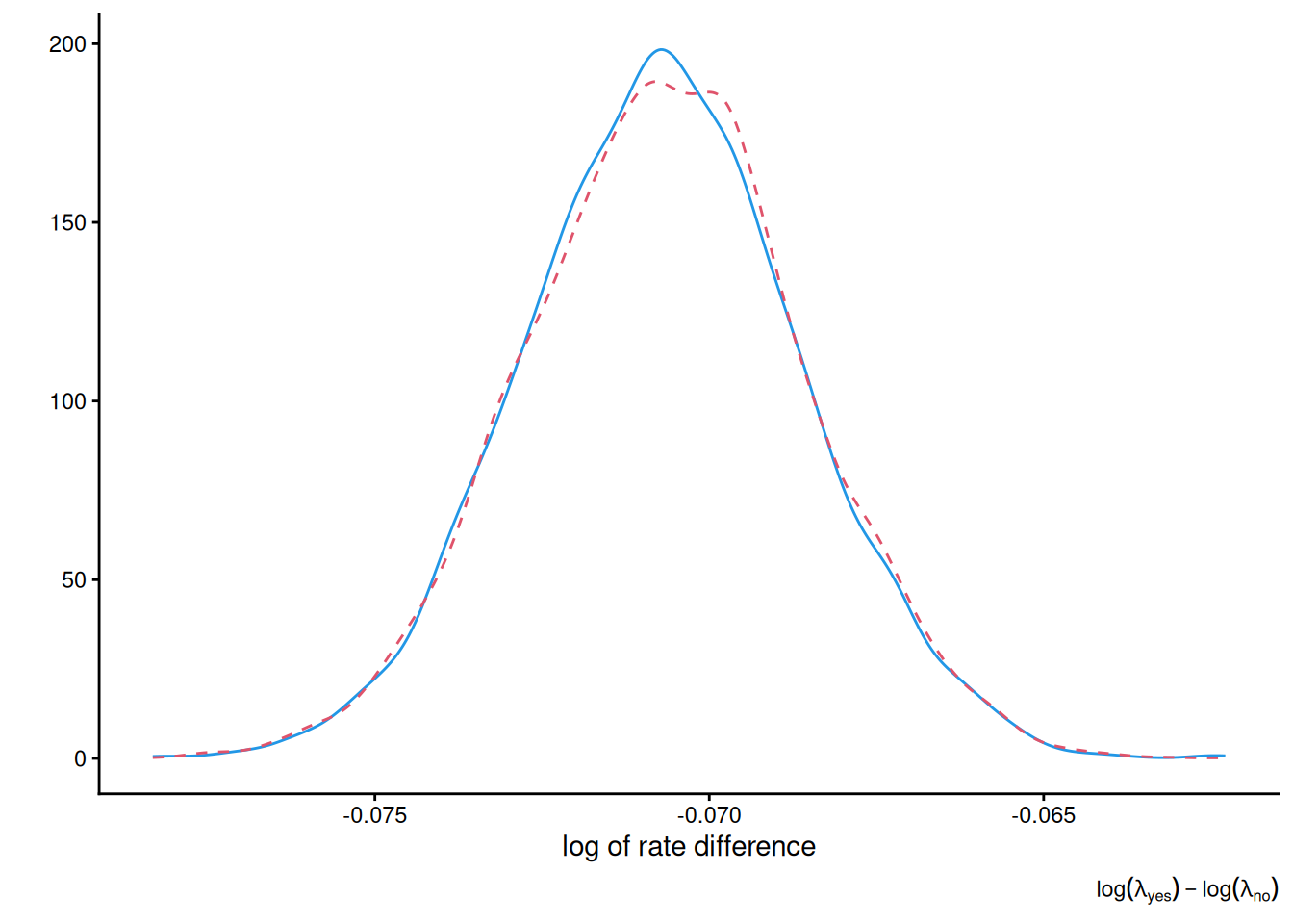

Figure 1: Posterior for the difference in mean for the Poisson regression model (blue) and the same model with an informative conjugate gamma prior (red).

We can use the priorsense package to perform a sensitivity analysis of the regression parameter for the log mean difference. The results here indicate little impact of the prior, which is totally unsurprising given the sample size.

priorsense::powerscale_sensitivity(headline_mod)

Sensitivity based on cjs_dist
Prior selection: all priors
Likelihood selection: all data

      variable prior likelihood diagnosis
 b_questionyes     0      0.081         -
  b_questionno     0      0.080         -

priorsense::powerscale_plot_dens(headline_mod)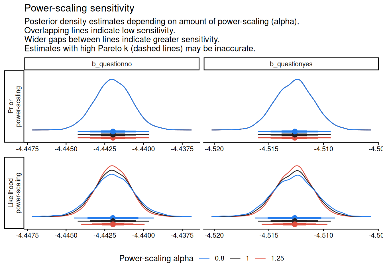

Figure 2: Prior sensitivity analysis and density of the posterior for different values of the powered prior.

Distraction from smartwatches

The following code is Stan code (mean-centered for the random effect) for the Poisson “mixed effect” model of Brodeur et al. (2021).

data {
  int<lower=0> N;
  int<lower=1> K; // nb fixed effect levels for distraction type
  int<lower=1> J; // nb random effect levels for individuals
  array[N] int<lower=0> y;    // vector of data
  array[N] int<lower=1, upper=J> id;
  array[N] int<lower=1, upper=K> fixed;
}
parameters {
  vector[K] beta;
   sum_to_zero_vector[J] alpha;
  real<lower=0> kappa;
}

model {
  kappa ~ exponential(0.6);
  beta ~ normal(0, 10);
  alpha ~ normal(0, sqrt(J * inv(J - 1)) * kappa);
  y ~ poisson_log(alpha[id] + beta[fixed]);
}

but this model is also easily fitted in brms, albeit with slightly different priors.

data(smartwatch, package = "hecbayes")
# Random effect model with default priors
smartwatch_mod <- brm(
  nviolation ~ 0 + task + (1 | id),
  data = smartwatch,
  family = poisson(link = "log"),
  set_prior(
    prior = "normal(0, 5)", 
    class = "b"),
  backend = "cmdstanr", # faster than rstan
  silent = 2) # remove verbose output
summary(smartwatch_mod)

 Family: poisson 
  Links: mu = log 
Formula: nviolation ~ 0 + task + (1 | id) 
   Data: smartwatch (Number of observations: 124) 
  Draws: 4 chains, each with iter = 2000; warmup = 1000; thin = 1;
         total post-warmup draws = 4000

Multilevel Hyperparameters:
~id (Number of levels: 31) 
              Estimate Est.Error l-95% CI u-95% CI Rhat Bulk_ESS Tail_ESS
sd(Intercept)     0.56      0.08     0.42     0.75 1.00      885     1777

Regression Coefficients:
            Estimate Est.Error l-95% CI u-95% CI Rhat Bulk_ESS Tail_ESS
taskphone       1.77      0.12     1.52     2.02 1.01      631     1237
taskwatch       1.73      0.13     1.48     1.98 1.01      624      982
taskspeaker     1.79      0.13     1.54     2.03 1.01      618     1184
tasktexting     2.43      0.11     2.20     2.65 1.01      543      970

Draws were sampled using sample(hmc). For each parameter, Bulk_ESS
and Tail_ESS are effective sample size measures, and Rhat is the potential
scale reduction factor on split chains (at convergence, Rhat = 1).

fixef(smartwatch_mod)

            Estimate Est.Error     Q2.5    Q97.5
taskphone   1.769084 0.1247112 1.521574 2.015402
taskwatch   1.731203 0.1254586 1.483068 1.975162
taskspeaker 1.793016 0.1253032 1.538412 2.032189
tasktexting 2.433497 0.1146008 2.203393 2.648241

conditional_effects(x = smartwatch_mod,
                    effects =  "task",
                    prob = 0.8)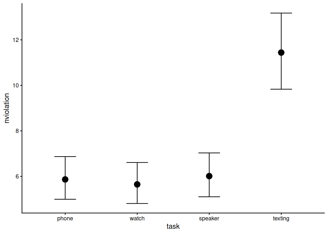

Climate change mean temperature increase

Different climate models and runs give rise to different average estimates of temperature increase. We can consider a very simple hierarchical model to capture this, assuming that data are Gaussian with model-specific “random effects”. The data are unbalanced: some climate models offer a single run, other mutliples.

library(bang) # Bayesian analysis with ROU
data(temp2)
RCP26 <- temp2 |> dplyr::filter(RCP == "rcp26")
anova_mod1 <- bang::hanova1(
  resp = RCP26$index,
  prior = "bda", # uniform on mu, log(sigma), sigma_a
  fac = RCP26$GCM)
anova_mod2 <- bang::hanova1(
  resp = RCP26$index,
  prior = "unif", # uniform on mu, sigma, sigma_a
  fac = RCP26$GCM)
anova_mod3 <- bang::hanova1(
  resp = RCP26$index,
  prior = "cauchy", # half-Cauchy  for the scale
  fac = RCP26$GCM)

The model is of the form, for \(r = 1, \ldots, R\): \[ Y_{i(r),r} \sim \mathsf{Gauss}(\mu + \alpha_r, \sigma^2), \alpha_r \sim \mathsf{Gauss}(0, \sigma^2_\alpha) \] and we need a prior \(p(\mu, \sigma_{\alpha}, \sigma).\) There are numerous priors that could be considered here.

• \(p(\mu, \sigma_{\alpha}, \sigma) \propto \sigma^{-1}\) (location-scale, improper if \(R < 3.\)
• \(p(\mu, \sigma_{\alpha}, \sigma) \propto 1\) (improper)
• \(p(\mu, \sigma_{\alpha}, \sigma) \propto (1+\sigma^2_{\alpha}/S_{\alpha}^2)^{-1}(1+\sigma^2/S^2)^{-1}\) on \(\mathbb{R} \times [0,\infty)^2.\) This corresponds to half-Cauchy distribution on the positive reals with a scale of \(S\) and \(S_{\alpha}\) (default 10).

Below, we plot the posterior density for each of the \(\alpha_r\) \((r=1, \ldots, R)\) for each of the three priors. There appears to be little difference to the first level, even for factor levels with few observations. Changing altogether the prior on the “random effect” from Gaussian to Cauchy would have more impact, as there is inherently a lot of regularization due to the prior in this specific application.

summary(anova_mod1,
        which_pop = c("theta[1]", "theta[8]"),
        params = "pop")

    theta[1]         theta[8]    
 Min.   :0.9415   Min.   :1.485  
 1st Qu.:1.0875   1st Qu.:1.546  
 Median :1.1280   Median :1.557  
 Mean   :1.1264   Mean   :1.557  
 3rd Qu.:1.1650   3rd Qu.:1.569  
 Max.   :1.3788   Max.   :1.621  

summary(anova_mod1,
        params = "hyper")

ru bounding box:  
               box         vals1        vals2 conv
a        1.0000000  0.0000000000  0.000000000    0
b1minus -0.1466810 -0.2326509993  0.001997345    0
b2minus -0.1475368 -0.0004397797 -0.234538810    0
b1plus   0.1755008  0.3048045193  0.001126515    0
b2plus   0.1739269 -0.0010104517  0.300416382    0

estimated probability of acceptance:  
[1] 0.5167959

sample summary 
       mu          sigma[alpha]        sigma        
 Min.   :0.8903   Min.   :0.2823   Min.   :0.04121  
 1st Qu.:1.1817   1st Qu.:0.4012   1st Qu.:0.05233  
 Median :1.2458   Median :0.4402   Median :0.05605  
 Mean   :1.2408   Mean   :0.4490   Mean   :0.05698  
 3rd Qu.:1.3007   3rd Qu.:0.4885   3rd Qu.:0.06113  
 Max.   :1.5148   Max.   :0.7210   Max.   :0.09077  

ggplot() +
  geom_density(
    data = anova_mod1$theta_sim_vals |>
      as.data.frame() |>
      tidyr::pivot_longer(
        cols = everything(),
        names_to = "GCM",
        values_to = "post"),
    mapping = aes(x = post, group = GCM))  +
  geom_density(
    data = anova_mod3$theta_sim_vals |>
      as.data.frame() |>
      tidyr::pivot_longer(
        cols = everything(),
        names_to = "GCM",
        values_to = "post"),
    mapping = aes(x = post, group = GCM),
    col = "#ef8a47")  +
  geom_density(
    data = anova_mod2$theta_sim_vals |>
      as.data.frame() |>
      tidyr::pivot_longer(
        cols = everything(),
        names_to = "GCM",
        values_to = "post"),
    mapping = aes(x = post, group = GCM),
    col = "#72bcd5")  +
  labs(x = "posterior mean") +
  theme_classic() +
  theme(legend.position = "none")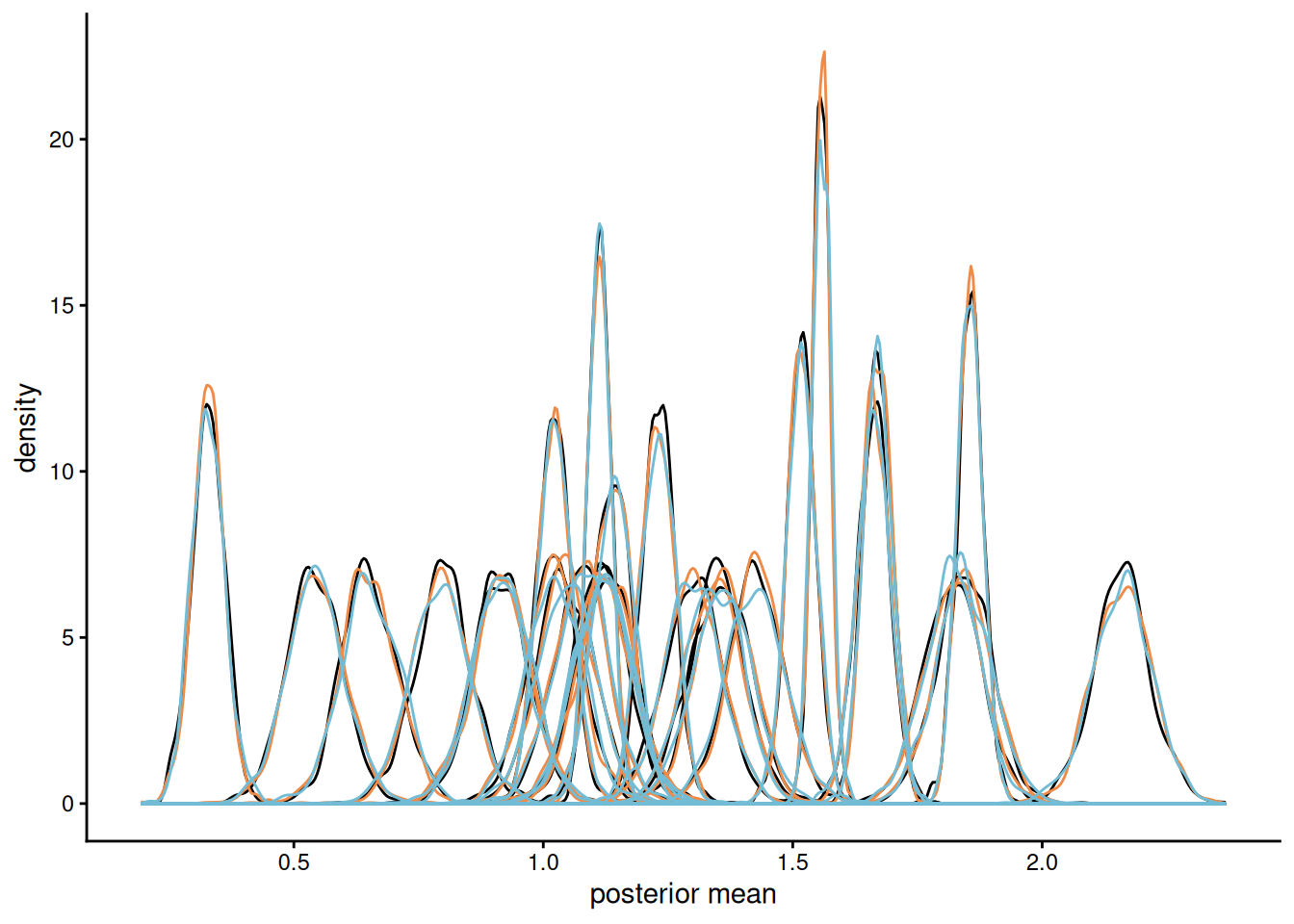

References

Brodeur, M., Ruer, P., Léger, P.-M., & Sénécal, S. (2021). Smartwatches are more distracting than mobile phones while driving: Results from an experimental study. Accident Analysis & Prevention, 149, 105846. https://doi.org/10.1016/j.aap.2020.105846