Bayesian modelling

Distribution and density function

Let $X \in R^{d}$ be a random vector with distribution function $\begin{array}{r} F_{X} (x) = Pr (X \leq x) = Pr (X_{1} \leq x_{1}, \dots, X_{d} \leq x_{d}) . \end{array}$

If the distribution of $X$ is absolutely continuous, $\begin{array}{r} F_{X} (x) = \int_{- \infty}^{x_{d}} \dots \int_{- \infty}^{x_{1}} f_{X} (z_{1}, \dots, z_{d}) d z_{1} \dots d z_{d}, \end{array}$ where $f_{X} (x)$ is the joint density function.

Mass function

By abuse of notation, we denote the mass function in the discrete case $0 \leq f_{X} (x) = Pr (X_{1} = x_{1}, \dots, X_{d} = x_{d}) \leq 1.$

The support is the set of non-zero density/probability total probability over all points in the support, $\sum_{x \in supp (X)} f_{X} (x) = 1.$

Marginal distribution

The marginal distribution of a subvector $X_{1 : k} = (X_{1}, \dots, X_{k})^{⊤}$ is $\begin{aligned} F_{X_{1 : k}} (x_{1 : k}) & = Pr (X_{1 : k} \leq x_{1 : k}) \\ = F_{X} (x_{1}, \dots, x_{k}, \infty, \dots, \infty) . \end{aligned}$

Marginal density

The marginal density $f_{X_{1 : k}} (x_{1 : k})$ of an absolutely continuous subvector $X_{1 : k} = (X_{1}, \dots, X_{k})^{⊤}$ is $\begin{array}{r} \int_{- \infty}^{\infty} \dots \int_{- \infty}^{\infty} f_{X} (x_{1}, \dots, x_{k}, z_{k + 1}, \dots, z_{d}) d z_{k + 1} \dots d z_{d} . \end{array}$ through integration from the joint density.

Conditional distribution

The conditional distribution function of $Y$ given $X = x$ , is $\begin{array}{r} f_{Y ∣ X} (y; x) = \frac{f_{X, Y} (x, y)}{f_{X} (x)} \end{array}$ for any value of $x$ in the support of $X$ .

Conditional and marginal for contingency table

Consider a bivariate distribution for $(Y_{1}, Y_{2})$ supported on ${1, 2, 3} \times {1, 2}$ whose joint probability mass function is given in Table 1

Table 1: Bivariate mass function with probability of each outcome for

(Y_{1}, Y_{2})

.

	$Y_{1} = 1$	$Y_{1} = 2$	$Y_{1} = 3$	row total
$Y_{2} = 1$	0.20	0.3	0.10	0.6
$Y_{2} = 2$	0.15	0.2	0.05	0.4
col. total	0.35	0.5	0.15	1.0

Calculations for the marginal distribution

The marginal distribution of $Y_{1}$ is obtain by looking at the total probability for each row/column, e.g., $Pr (Y_{1} = i) = Pr (Y_{1} = i, Y_{2} = 1) + Pr (Y_{1} = i, Y_{2} = 2) .$

$Pr (Y_{1} = 1) = 0.35$ , $Pr (Y_{1} = 2) = 0.5$ , $Pr (Y_{1} = 3) = 0.15$ .
$Pr (Y_{2} = 1) = 0.6$ and $Pr (Y_{2} = 2) = 0.4$

Conditional distribution

The conditional distribution $Pr (Y_{2} = i ∣ Y_{1} = 2) = \frac{Pr (Y_{1} = 2, Y_{2} = i)}{Pr (Y_{1} = 2)},$ so $\begin{aligned} Pr (Y_{2} = 1 ∣ Y_{1} = 2) & = 0.3 / 0.5 = 0.6 \\ Pr (Y_{2} = 2 ∣ Y_{1} = 2) & = 0.4 . \end{aligned}$

Independence

Vectors $Y$ and $X$ are independent if $\begin{array}{r} F_{X, Y} (x, y) = F_{X} (x) F_{Y} (y) \end{array}$ for any value of $x$ , $y$ .

The joint density, if it exists, also factorizes $\begin{array}{r} f_{X, Y} (x, y) = f_{X} (x) f_{Y} (y) . \end{array}$

If two subvectors $X$ and $Y$ are independent, then the conditional density $f_{Y ∣ X} (y; x)$ equals the marginal $f_{Y} (y)$ .

Expected value

If $Y$ has density $f_{Y},$ then $\begin{array}{r} E {g (Y)} = \int g (y) f_{Y} (y) d y \end{array}$ a weighted integral of $g$ with weight $f_{Y} .$

The identity function gives the expected value $E (Y) .$

Covariance matrix

We define the covariance matrix of $Y$ as $\begin{array}{r} Va (Y) = E [{Y - E (Y)} {Y - E (Y)}^{⊤}], \end{array}$ which reduces in the unidimensional setting to $Va (Y) = E {Y - E (Y)}^{2} = E (Y^{2}) - E (Y)^{2} .$

Affine transformations

If $Y$ is $d$ -dimensional and $A$ is $p \times d$ and $b$ is a $p$ vector, then

$\begin{aligned} E (A Y + b) & = A E (Y) + b, \\ Va (A Y + b) & = A Va (Y) A^{⊤} . \end{aligned}$

Law of iterated expectation and variance

Let $Z$ and $Y$ be random vectors. The expected value of $Y$ is $\begin{array}{r} E_{Y} (Y) = E_{Z} {E_{Y ∣ Z} (Y)} . \end{array}$

The tower property gives a law of iterated variance $\begin{array}{r} {Va}_{Y} (Y) = E_{Z} {{Va}_{Y ∣ Z} (Y)} + {Va}_{Z} {E_{Y ∣ Z} (Y)} . \end{array}$

Poisson distribution

The Poisson distribution has mass $\begin{array}{r} f (x) = \Pr (Y = x) = \frac{\exp (- λ) λ^{y}}{Γ (y + 1)}, x = 0, 1, 2, \dots \end{array}$ where $Γ (\cdot)$ denotes the gamma function.

The parameter $λ$ of the Poisson distribution is both the expectation and the variance of the distribution, meaning $E (Y) = Va (Y) = λ .$

Gamma distribution

A gamma distribution with shape $α > 0$ and rate $β > 0$ , denoted $Y \sim gamma (α, β)$ , has density $\begin{array}{r} f (x) = \frac{β^{α}}{Γ (α)} x^{α - 1} \exp (- β x), x \in (0, \infty), \end{array}$ where $Γ (α) = \int_{0}^{\infty} t^{α - 1} \exp (- t) d t$ is the gamma function.

Poisson with random scale

To handle overdispersion in count data, take

$\begin{aligned} Y ∣ Λ & = λ \sim Poisson (λ) \\ Λ & \sim Gamma (k μ, k) . \end{aligned}$

The joint density of $Y$ and $Λ$ on $N = {0, 1, \dots} \times R_{+}$ is $\begin{aligned} f (y, λ) & = f (y ∣ λ) f (λ) \\ = \frac{λ^{y} \exp (- λ)}{Γ (y + 1)} \frac{k^{k μ} λ^{k μ - 1} \exp (- k λ)}{Γ (k μ)} \end{aligned}$

Conditional distribution

The conditional distribution of $Λ ∣ Y = y$ can be found by considering only terms that are function of $λ$ , whence $\begin{array}{r} f (λ ∣ Y = y) \overset{λ}{\propto} λ^{y + k μ - 1} \exp {- (k + 1) λ} \end{array}$ so $Λ ∣ Y = y \sim gamma (k μ + y, k + 1)$ .

Marginal density of Poisson mean mixture

$\begin{aligned} f (y) & = \frac{f (y, λ)}{f (λ ∣ y)} = \frac{\frac{λ^{y} \exp (- λ)}{Γ (y + 1)} \frac{k^{k μ} λ^{k μ - 1} \exp (- k λ)}{Γ (k μ)}}{\frac{(k + 1)^{k μ + y} λ^{k μ + y - 1} \exp {- (k + 1) λ}}{Γ (k μ + y)}} \\ = \frac{Γ (k μ + y)}{Γ (k μ) Γ (y + 1)} k^{k μ} (k + 1)^{- k μ - y} \\ = \frac{Γ (k μ + y)}{Γ (k μ) Γ (y + 1)} {(1 - \frac{1}{k + 1})}^{k μ} {(\frac{1}{k + 1})}^{y} \end{aligned}$ Marginally, $Y \sim neg . binom (p)$ where $p = (k + 1)^{- 1} .$

Moments of negative binomial

By the laws of iterated expectation and iterative variance, $\begin{aligned} E (Y) & = E_{Λ} {E (Y ∣ Λ} \\ = E (Λ) = μ \\ Va (Y) & = E_{Λ} {Va (Y ∣ Λ)} + {Va}_{Λ} {E (Y ∣ Λ)} \\ = E (Λ) + Va (Λ) \\ = μ + μ / k . \end{aligned}$ The marginal distribution of $Y$ , unconditionally, has a variance which exceeds its mean.

Change of variable formula

Consider an injective (one-to-one) differentiable function $g : R^{d} \to R^{d},$ with inverse $g^{- 1} .$ Then, if $Y = g (X),$ $\begin{array}{r} Pr (Y \leq y) = Pr {g (X) \leq y} = Pr {X \leq x = g^{- 1} (y)} . \end{array}$

Using the chain rule, the density of $Y$ is $\begin{array}{r} f_{Y} (y) = f_{X} {g^{- 1} (y)} | J_{g^{- 1}} (y) | = f_{X} (x) {| J_{g} (x) |}^{- 1} \end{array}$ where $J_{g} (x)$ is the Jacobian matrix with $i, j$ th element $\partial [g (x)]_{i} / \partial x_{j} .$

Gaussian location-scale

Consider $d$ independent standard Gaussian variates $X_{j} \sim Gauss (0, 1)$ for $j = 1, \dots, d,$ with joint density function $\begin{array}{r} f_{X} (x) = (2 π)^{- d / 2} \exp (- \frac{x^{⊤} x}{2}) . \end{array}$ Consider the transformation $Y = A X + b,$ with $A$ an invertible matrix.

Change of variable for Gaussian

The inverse transformation is $g^{- 1} (y) = A^{- 1} (y - b) .$
The Jacobian $J_{g} (x)$ is simply $A,$ so the joint density of $Y$ is $\begin{array}{r} (2 π)^{- d / 2} | A |^{- 1} \exp {- \frac{(y - b)^{⊤} A^{- ⊤} A^{- 1} (y - b)}{2}} . \end{array}$ Since $| A^{- 1} | = | A |^{- 1}$ and $A^{- ⊤} A^{- 1} = ({AA}^{⊤})^{- 1},$ we recover $Y \sim {Gauss}_{d} (b, {AA}^{⊤}) .$

Conditional distribution of Gaussian subvectors

Let $Y \sim {Gauss}_{d} (μ, Q^{- 1})$ and consider the partition $\begin{array}{r} Y = (\begin{array}{c} Y_{1} \\ Y_{2} \end{array}), μ = (\begin{array}{c} μ_{1} \\ μ_{2} \end{array}), Q = (\begin{array}{c} Q_{11} & Q_{12} \\ Q_{21} & Σ_{22} \end{array}), \end{array}$ where $Y_{1}$ is a $k \times 1$ and $Y_{2}$ is a $(d - k) \times 1$ vector for some $1 \leq k < d .$

Then, we have the conditional distribution $\begin{aligned} Y_{1} ∣ Y_{2} = y_{2} & \sim {Gauss}_{k} (μ_{1} - Q_{11}^{- 1} Q_{12} (y_{2} - μ_{2}), Q_{11}^{- 1}) \end{aligned}$

Likelihood

The likelihood $L (θ)$ is a function of the parameter vector $θ$ that gives the ‘density’ of a sample under a postulated distribution, treating the observations as fixed, $\begin{array}{r} L (θ; y) = f (y; θ) . \end{array}$

Likelihood for independent observations

If the joint density factorizes, $\begin{array}{r} L (θ; y) = \prod_{i = 1}^{n} f_{i} (y_{i}; θ) = f_{1} (y_{1}; θ) \times \dots \times f_{n} (y_{n}; θ) . \end{array}$ The corresponding log likelihood function for independent and identically distributions observations is $\begin{array}{r} ℓ (θ; y) = \sum_{i = 1}^{n} \ln f (y_{i}; θ) \end{array}$

Score

Let $ℓ (θ),$ $θ \in Θ \subseteq R^{p},$ be the log likelihood function. The gradient of the log likelihood, termed score is the $p$ -vector $U (θ) = \frac{\partial ℓ (θ)}{\partial θ} .$

Information matrix

The observed information matrix is the hessian of the negative log likelihood, $\begin{array}{r} j (θ; y) = - \frac{\partial^{2} ℓ (θ; y)}{\partial θ \partial θ^{⊤}}, \end{array}$ evaluated at the maximum likelihood estimate $\hat{θ},$ so $j (\hat{θ}) .$

Expected information

Under regularity conditions, the expected information, also called Fisher information matrix, is $\begin{array}{r} i (θ) = E {U (θ; Y) U (θ; Y)^{⊤}} = E {j (θ; Y)} \end{array}$

Note on information matrices

Information matrices are symmetric and provide information about the variability of $\hat{θ} .$

The information of an iid sample of size $n$ is $n$ times that of a single observation

information accumulates at a linear rate.

Information for the Gaussian distribution

Consider $Y \sim Gauss (μ, τ^{- 1})$ , parametrized in terms of precision $τ$ . The likelihood contribution for an $n$ sample is, up to proportionality, $\begin{array}{r} ℓ (μ, τ) \propto \frac{n}{2} \log (τ) - \frac{τ}{2} \sum_{i = 1}^{n} (Y_{i}^{2} - 2 μ Y_{i} + μ^{2}) \end{array}$

Gaussian information matrices

The observed and Fisher information matrices are $\begin{aligned} j (μ, τ) & = (\begin{array}{c} n τ & - \sum_{i = 1}^{n} (Y_{i} - μ) \\ - \sum_{i = 1}^{n} (Y_{i} - μ) & \frac{n}{2 τ^{2}} \end{array}), \\ i (μ, τ) & = n (\begin{array}{c} τ & 0 \\ 0 & \frac{1}{2 τ^{2}} \end{array}) \end{aligned}$ Since $E (Y_{i}) = μ$ , the expected value of the off-diagonal entries of the Fisher information matrix are zero.

Example: random right-censoring

Consider a survival analysis problem for independent time-to-event data subject to (noninformative) random right-censoring. We observe

failure times $Y_{i} (i = 1, \dots, n)$ drawn from $F (\cdot; θ)$ supported on $(0, \infty)$
independent binary censoring indicators $C_{i} \in {0, 1}$ , with $0$ indicating right-censoring and $C_{i} = 1$ observed failure time.

Likelihood contribution with censoring

If individual observation $i$ has not experienced the event at the end of the collection period, then the likelihood contribution is $Pr (Y > y) = 1 - F (y; θ)$ , where $y_{i}$ is the maximum time observed for $Y_{i}$ . We write the log likelihood $\begin{array}{r} ℓ (θ) = \sum_{i : c_{i} = 0} \log {1 - F (y_{i}; θ)} + \sum_{i : c_{i} = 1} \log f (y_{i}; θ) \end{array}$

Censoring and exponential data

Suppose for simplicity that $Y_{i} \sim expo (λ)$ and let $m = c_{1} + \dots + c_{n}$ denote the number of observed failure times. Then, the log likelihood and the Fisher information are $\begin{aligned} ℓ (λ) & = λ \sum_{i = 1}^{n} y_{i} + \log λ m \\ i (λ) & = m / λ^{2} \end{aligned}$ and the right-censored observations for the exponential model do not contribute to the information.

Example: first-order autoregressive process

Consider an $AR (1)$ model of the form $Y_{t} = μ + ϕ (Y_{t - 1} - μ) + ε_{t},$ where

$ϕ$ is the lag-one correlation,
$μ$ the global mean and
$ε_{t}$ is an iid innovation with mean zero and variance $σ^{2}$ .

If $| ϕ | < 1$ , the process is stationary, and the variance does not increase with $t$ .

Markov property and likelihood decomposition

The Markov property states that the current realization depends on the past, $Y_{t} ∣ Y_{1}, \dots, Y_{t - 1},$ only through the most recent value $Y_{t - 1} .$ The log likelihood thus becomes $\begin{array}{r} ℓ (θ) = \ln f (y_{1}) + \sum_{i = 2}^{n} f (y_{i} ∣ y_{i - 1}) . \end{array}$

Marginal of AR(1)

The $AR (1)$ stationarity process has unconditional moments $E (Y_{t}) = μ, Var (Y_{t}) = σ^{2} / (1 - ϕ^{2}) .$

The $AR (1)$ process is first-order Markov since the conditional distribution $f (Y_{t} ∣ Y_{t - 1}, \dots, Y_{t - p})$ equals $f (Y_{t} ∣ Y_{t - 1})$ .

Log likelihood of AR(1)

If innovations are Gaussian, we have $Y_{t} ∣ Y_{t - 1} = y_{t - 1} \sim Gauss {μ (1 - ϕ) + ϕ y_{t - 1}, σ^{2}}, t > 1.$ so the log-likelihood is $\begin{aligned} ℓ (μ, ϕ, σ^{2}) = - \frac{n}{2} \log (2 π) - n \log σ + \frac{1}{2} \log (1 - ϕ^{2}) \\ - \frac{(1 - ϕ^{2}) (y_{1} - μ)^{2}}{2 σ^{2}} - \sum_{i = 2}^{n} \frac{(y_{t} - μ (1 - ϕ) - ϕ y_{t - 1})^{2}}{2 σ^{2}} \end{aligned}$

Estimation of integrals

Suppose we can simulate $B$ i.i.d. variables with the same distribution, $x_{1}, \dots, x_{B}$ with distribution $F$ .

We want to compute $E {g (X)} = \int g (x) f (x) d x = μ_{g}$ for some functional $g (\cdot)$

$g (x) = x$ (mean)
$g (x) = I (x \in A)$ (probability of event)
etc.

Vanilla Monte Carlo integration

We substitute expected value by sample average of $\begin{array}{r} {\hat{μ}}_{g} = \frac{1}{B} \sum_{b = 1}^{B} g (x_{b}) . \end{array}$

law of large number guarantees convergence of ${\hat{μ}}_{g} \to μ_{g}$ if the latter is finite.
Under finite second moments, central limit theorem gives $\sqrt{B} ({\hat{μ}}_{g} - μ_{g}) \sim No (0, σ_{g}^{2}) .$

Importance sampling

Consider density $q$ instead with $supp (p) \subseteq supp (q) .$ Then, $\begin{array}{r} E {g (X)} = \int_{X} g (x) \frac{p (x)}{q (x)} q (x) d x \end{array}$ and we can proceed similarly by drawing samples from $q$ .

Importance sampling estimator

An alternative Monte Carlo estimator uses the weighted average $\begin{array}{r} \tilde{E} {g (X)} = \frac{B^{- 1} \sum_{b = 1}^{B} w_{b} g (x_{b})}{B^{- 1} \sum_{b = 1}^{B} w_{b}} . \end{array}$ with weights $w_{b} = p (x_{b}) / q (x_{b})$ . The latter equal 1 on average, so one could omit the denominator without harm.

Standard errors

If the variance of $g (X)$ is finite, we can approximate the latter by the sample variance of the simple random sample and obtain the Monte Carlo standard error of the estimator $\begin{array}{r} {se}^{2} [\hat{E} {g (X)}] = \frac{1}{B (B - 1)} \sum_{b = 1}^{B} {[g (x_{b}) - \hat{E} {g (X)}]}^{2} . \end{array}$

Precision of Monte Carlo integration

We want to have an estimator as precise as possible.

but we can’t control the variance of $g (X)$ , say $σ_{g}^{2}$
the more simulations $B$ , the lower the variance of the mean.
sample average for i.i.d. data has variance $σ_{g}^{2} / B$
to reduce the standard deviation by a factor 10, we need $100$ times more draws!

Remember: the answer is random.

Example: functionals of gamma distribution

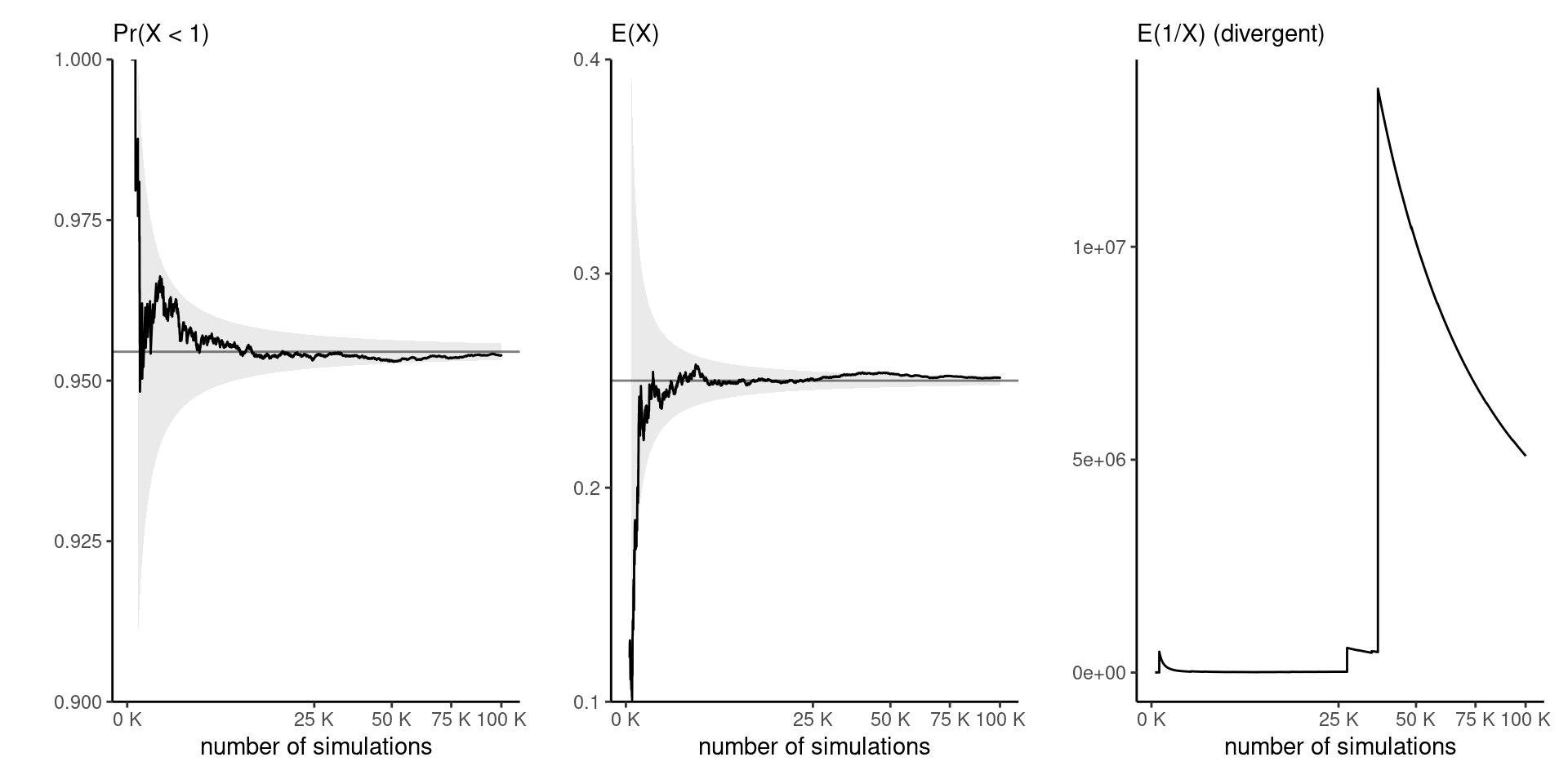
Figure 1: Running mean trace plots for $g (x) = I (x < 1)$ (left), $g (x) = x$ (middle) and $g (x) = 1 / x$ (right) for a Gamma distribution with shape 0.5 and rate 2, as a function of the Monte Carlo sample size.

Recap

We can specify distribution using hierarchies, with marginal $\times$ conditional.
Most density and mass functions for $Y$ can be identified from their support and their kernel, i.e., terms that depend on $y$ , ignoring normalizing constants. We then match expressions.
Expectations can be calculated analytically, or approximated via Monte Carlo simulations.