Bayesian modelling

Priors

The posterior density is

$\begin{array}{r} p (θ ∣ Y) = \frac{p (Y ∣ θ) \times p (θ)}{\int p (Y ∣ θ) p (θ) d θ}, \end{array}$

where $posterior \propto likelihood \times prior$

We need to determine a suitable prior.

Impact of the prior

The posterior is a compromise prior and likelihood:

the more informative the prior, the more the posterior resembles it.
in large samples, the effect of the prior is often negligible

Controversial?

No unique choice for the prior: different analysts get different inferences
What is the robustness to the prior specification? Check through sensitivity analysis.
Even with prior knowledge, hard to elicit parameter (many different models could yield similar summary statistics)

Choosing priors

Infinite number of choice, but many default choices…

conditionally conjugate priors (ease of interpretation, computational advantages)
flat priors and vague priors (mostly uninformative)
informative priors (expert opinion)
Jeffrey’s priors (improper, invariant to reparametrization)
penalized complexity (regularization)
shrinkage priors (variable selection, reduce overfitting)

Determining hyperparameters

We term hyperparameters the parameters of the (hyper)priors.

How to elicit reasonable values for them?

use moment matching to get sensible values
trial-and-error using the prior predictive
- draw a parameter value from the prior $θ_{0}$
- for each, generate a new observation from the model $f (y_{new} ∣ θ_{0})$

Example of simple linear regression

Working with standardized response and inputs $x_{i} \mapsto (x_{i} - \overset{―}{x}) / sd (x),$

the slope is the correlation between explanatory $X$ and response $Y$
the intercept should be mean zero
are there sensible bounds for the range of the response?

Example - simple linear regression

Consider the relationship between height ( $Y,$ in cm) and weight ( $X,$ in kg) among humans adults.¹

Model using a simple linear regression

$\begin{aligned} Y_{i} & \sim Gauss (μ_{i}, σ^{2}) \\ μ_{i} & = β_{0} + β_{1} (x_{i} - \overset{―}{x}) \\ β_{0} & \sim Gauss (178, 20^{2}) \\ σ & \sim unif (0, 50) \end{aligned}$ What about the slope parameter prior $p (β_{1})$ ?

Priors for the slope

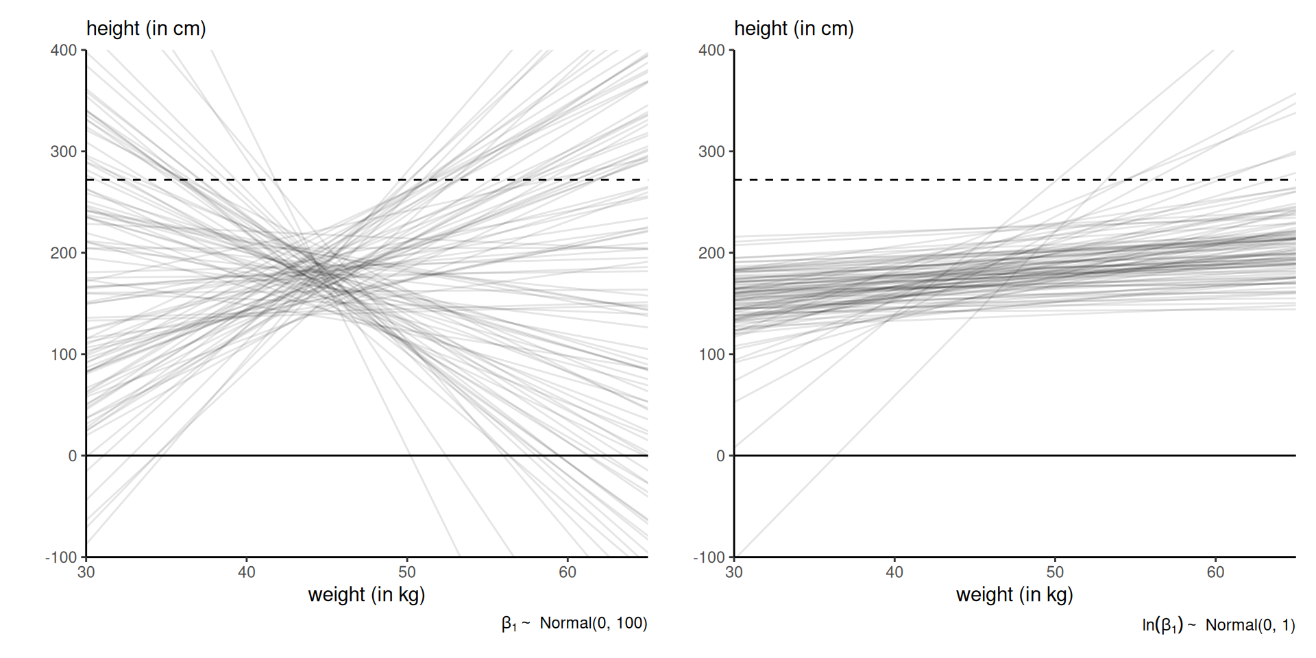
Figure 1: Prior draws of linear regressions with different priors: vague $β_{1} \sim Gauss (0, 100)$ (left) and lognormal $\ln (β_{1}) \sim Gauss (0, 1)$ (right). Figure 4.5 of McElreath (2020). The Guiness record for the world’s tallest person is 272cm.

Conjugate priors

A prior density $p (θ)$ is conjugate for likelihood $L (θ; y)$ if the product $L (θ; y) p (θ),$ after renormalization, is of the same parametric family as the prior.

Distributions that are exponential family admit conjugate priors.

A distribution is an exponential family if it’s density can be written $\begin{array}{r} f (y; θ) = \exp {\sum_{k = 1}^{K} Q_{k} (θ) t_{k} (y) + D (θ) + h (y)} . \end{array}$ The support of $f$ must not depend on $θ .$

Conjugate priors for common exponential families

distribution	unknown parameter	conjugate prior
$Y \sim expo (λ)$	$λ$	$λ \sim gamma (α, β)$
$Y \sim Poisson (μ)$	$μ$	$μ \sim gamma (α, β)$
$Y \sim binom (n, θ)$	$θ$	$θ \sim Be (α, β)$
$Y \sim Gauss (μ, σ^{2})$	$μ$	$μ \sim Gauss (ν, ω^{2})$
$Y \sim Gauss (μ, σ^{2})$	$σ$	$σ^{- 2} \sim gamma (α, β)$
$Y \sim Gauss (μ, σ^{2})$	$μ, σ$	$μ ∣ σ^{2} \sim Gauss (ν, ω σ^{2}),$ $σ^{- 2} \sim gamma (α, β)$

Conjugate prior for the Poisson

If $Y \sim Poisson (μ)$ with density $f (y) = μ^{x} \exp (- μ x) / x!,$ then for $μ \sim gamma (α, β)$ with $α, β$ fixed. Consider an i.i.d. sample with mean $\overset{―}{y} .$ The posterior density is

$p (μ ∣ y) \overset{μ}{\propto} μ^{n \overset{―}{y}} \exp (- μ n \overset{―}{y}) μ^{α - 1} \exp (- β μ)$ so must be gamma $gamma (n \overset{―}{y} + α, n \overset{―}{y} + β) .$

Parameter interpretation: $α$ events in $β$ time intervals.

Conjugate prior for Gaussian (known variance)

Consider an iid sample, $Y_{i} \sim Gauss (μ, σ^{2})$ and let $μ ∣ σ \sim Gauss (ν, σ^{2} τ^{2}) .$ Then, $\begin{aligned} p (μ, σ) & \propto \frac{p (σ)}{σ^{n + 1}} \exp {- \frac{1}{2 σ^{2}} \sum_{i = 1}^{n} (y_{i} - μ)^{2}} \exp {- \frac{1}{2 σ^{2} τ^{2}} (μ - ν)^{2}} \\ \propto \frac{p (σ)}{σ^{n + 1}} \exp {(\sum_{i = 1}^{n} y_{i} + \frac{ν}{τ^{2}}) \frac{μ}{σ^{2}} - (\frac{n}{2} + \frac{1}{2 τ^{2}}) \frac{μ^{2}}{σ^{2}}} . \end{aligned}$

The conditional posterior $p (μ ∣ σ)$ is Gaussian with

mean $(n \overset{―}{y} τ^{2} + ν) / (n τ^{2} + 1)$ and
precision (reciprocal variance) $(n + 1 / τ^{2}) / σ^{2} .$

Upworthy examples

The Upworthy Research Archive (Matias et al., 2021) contains results for 22743 experiments, with a click through rate of 1.58% on average and a standard deviation of 1.23%.
We consider an A/B test that compared four different headlines for a story.
We model the conversion rate for each using ${click}_{i} \sim Poisson (λ_{i} {impression}_{i}) .$

We treat $impression$ as a known offset.

Headlines

Consider an A/B test from November 23st, 2014, that compared four different headlines for a story on Sesame Street workshop with interviews of children whose parents were in jail and visiting them in prisons. The headlines tested were:

Some Don’t Like It When He Sees His Mom. But To Him? Pure Joy. Why Keep Her From Him?
They’re Not In Danger. They’re Right. See True Compassion From The Children Of The Incarcerated.
Kids Have No Place In Jail … But In This Case, They Totally Deserve It.
Going To Jail Should Be The Worst Part Of Their Life. It’s So Not. Not At All.

A/B test: Sesame street example

headline	impressions	clicks
H1	3060	49
H2	2982	20
H3	3112	31
H4	3083	9

Moment matching for gamma distribution

For $Y \sim gamma (α, β)$ with $β$ the rate parameter, we have $\begin{array}{r} E (Y) = α / β, Va (Y) = α / β^{2} . \end{array}$ We can solve for $β = E_{0} (λ) / {Va}_{0} (λ)$ and then use the mean relationship to retrieve $.

mu <- 0.0158; sd <- 0.0123
(beta <- mu/sd^2)

[1] 104.4352

(alpha <- mu * beta)

[1] 1.650076

Moment matching gives $α = 1.65$ and $β = 104.44 .$

Posterior distributions for Sesame Street

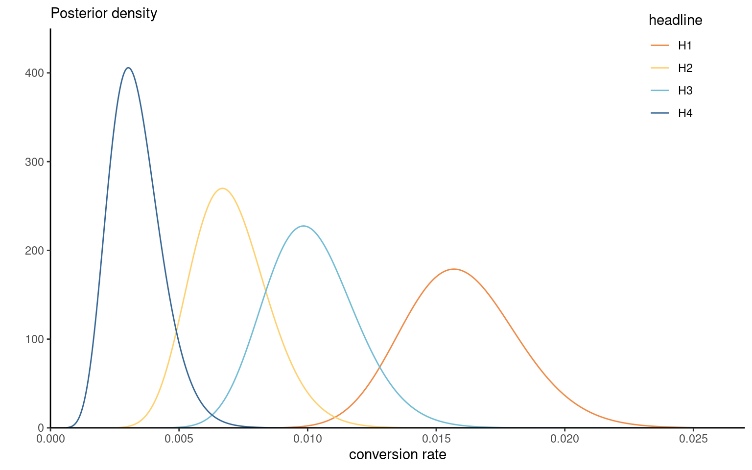
Figure 2: Gamma posteriors of the conversion rate for the Upworthy Sesame street headline.

Proper priors

Theorem 1 A sufficient condition for a prior to yield a proper (i.e., integrable) posterior density function is that it is (proportional) to a density function.

If we pick an improper prior, we need to check that the posterior is well-defined.
The answer to this question may depend on the sample size.

Proper posterior in a random effect model

Consider a Gaussian random effect model with $n$ independent observations in $J$ groups

The $i$ th observation in group $j$ is $\begin{aligned} Y_{i j} & \sim Gauss (μ_{i j}, σ^{2}) \\ μ_{i j} & = X_{i} β + α_{j}, \\ α_{j} & \sim Gauss (0, τ^{2}) \\ . . . \end{aligned}$

Conditions for a proper posterior

for $τ \sim unif (0, \infty),$ we need at least $J \geq 3$ ‘groups’ for the posterior to be proper.
if we take $p (τ) \propto τ^{- 1},$ the posterior is never proper.

As Gelman (2006) states:

in a hierarchical model the data can never rule out a group-level variance of zero, and so [a] prior distribution cannot put an infinite mass in this area

Improper priors as limiting cases

We can view the improper prior as a limiting case $σ \sim unif (0, t), t \to \infty .$

The Haldane prior for $θ$ in a binomial model is $θ^{- 1} (1 - θ)^{- 1},$ a limiting $Be (0, 0)$ distribution.

The improper prior $p (σ) \propto σ^{- 1}$ is equivalent to an inverse gamma $inv . gamma (ϵ, ϵ)$ when $ϵ \to 0.$

The limiting posterior is thus improper for random effects scales, so the value of $ϵ$ matters.

MDI prior for generalized Pareto

Let $Y_{i} \sim GP (σ, ξ)$ be generalized Pareto with density $f (x) = σ^{- 1} (1 + ξ x / σ)_{+}^{- 1 / ξ - 1}$ for $σ > 0$ and $ξ \in R,$ and $x_{+} = max {0, x} .$

Consider the maximum data information (MDI) $p (ξ) \propto \exp (- ξ) .$

Since $lim_{ξ \to - \infty} \exp (- ξ) = \infty,$ the prior density increases without bound as $ξ$ becomes smaller.

Truncated MDI for generalized Pareto distribution

The MDI prior leads to an improper posterior without modification.

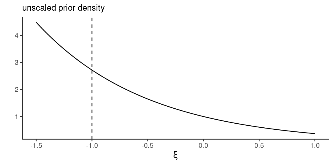
Figure 3: Unscaled maximum data information (MDI) prior density.

If we restrict the range of the MDI prior $p (ξ)$ to $ξ \geq - 1,$ then $p (ξ + 1) \sim expo (1)$ and posterior is proper.

Flat priors

Uniform prior over the support of $θ,$ $p (θ) \propto 1.$

Improper prior unless $θ \in [a, b]$ for finite $a, b .$

Flat priors for scale parameters

Consider a scale parameter $σ > 0.$

We could truncate the range, e.g., $σ \sim unif (0, 50),$ but this is not ‘uninformative’, as extreme values of $σ$ are as likely as small ones.
These priors are not invariant: if $p {\log (σ)} \propto 1$ implies $p (σ) \propto σ^{- 1}$ so can be informative on another scale.

Vague priors

Vague priors are very diffuse proper prior.

For example, a vague Gaussian prior for regression coefficients on standardized data, $β \sim {Gauss}_{p} (0_{p}, 100 I_{p}) .$

if we consider a logistic regression with a binary variable $X_{j} \in {0, 1},$ then $β_{j} = 5$ gives odds ratios of 150, and $β_{j} = 10$ of around 22K…

Invariance and Jeffrey’s prior

In single-parameter models, the Jeffrey’s prior $p (θ) \propto | ı (θ) |^{1 / 2},$ proportional to the square root of the determinant of the Fisher information matrix, is invariant to any (differentiable) reparametrization.

Jeffrey’s prior for the binomial distribution

Consider $Y \sim binom (1, θ) .$ The negative of the second derivative of the log likelihood with respect to $p$ is $ȷ (θ) = - \partial^{2} ℓ (θ; y) / \partial θ^{2} = y / θ^{2} + (1 - y) / (1 - θ)^{2} .$

Since $E (Y) = θ,$ the Fisher information is $ı (ϑ) = E {ȷ (θ)} = 1 / θ + 1 / (1 - θ) = 1 / {θ (1 - θ)} .$ Jeffrey’s prior is therefore $p (θ) \propto θ^{- 1 / 2} (1 - θ)^{- 1 / 2},$ a conjugate Beta prior $Be (0.5, 0.5) .$

Invariant priors for location-scale families

For a location-scale family with location $μ$ and scale $σ,$ the independent priors $\begin{aligned} p (μ) & \propto 1 \\ p (σ) & \propto σ^{- 1} \end{aligned}$ are location-scale invariant.

The results are invariant to affine transformations of the units, $ϑ = a + b θ .$

Penalized complexity priors

Simpson et al. (2017) consider a principled way of constructing priors that penalized model complexity for stable inference and limit over-specification.

Computes Kullback–Leibler divergence between $f$ and base model $f_{0}$ densities, builds an exponential prior on the distance scale and backtransform.

The resulting prior is scale-invariant, but it’s derivation is nontrivial.

Penalized complexity prior for random effect scale

If $α_{j} \sim Gauss (0, ζ^{2}),$ the penalized complexity prior for the scale $ζ \sim expo (λ) .$

Elicit $Q,$ a high quantile of the standard deviation $ζ$ with tail probability $α$ and set $λ = - \log (α / Q) .$

Priors for scale of random effects

The conjugate inverse gamma prior $p (ζ^{2}) \sim inv . gamma (α, β)$ is such that the mode for $ζ^{2}$ is $β / (1 + α) .$

Often, we take $β = α = 0.01$ or $0.001,$ but this leads to near-improper priors, so small values of the parameters are not optimal for ‘random effects’.

The inverse gamma prior cannot provide shrinkage or allow for no variability between groups.

Priors for scale of random effects

A popular suggestion, due to Gelman (2006), is to take a centered Student- $t$ distribution with $ν$ degrees of freedoms, truncated over $[0, \infty)$ with scale $s .$

since the mode is at zero, provides support for the base model
we want small degrees of freedom $ν,$ preferable to take $ν = 3$ ? Cauchy model ( $ν = 1$ ) still popular.

Prior sensitivity

Does the priors matter? As robustness check, one can fit the model with

different priors function
different hyperparameter values

Costly, but may be needed to convince reviewers ;)

Distraction from smartwach

We consider an experimental study conducted at Tech3Lab on road safety.

In Brodeur et al. (2021), 31 participants were asked to drive in a virtual environment.
The number of road violation was measured for 4 different type of distractions (phone notification, phone on speaker, texting and smartwatch).
Balanced data, random order of tasks

Poisson mixed model

We model the number of violations, nviolation as a function of distraction type (task) and participant id. $\begin{aligned} {nviolation}_{i j} & \sim Poisson (μ_{i j}) \\ μ_{i j} & = \exp (β_{j} + α_{i}), \\ β_{j} & \sim Gauss (0, 100), \\ α_{i} & \sim Gauss (0, τ^{2}) . \end{aligned}$

Specifically,

$β_{j}$ is the coefficient for task $j$ (distraction type),
$α_{i}$ is the random effect of participant $i .$

Priors for random effect scale

Consider different priors for $τ$

flat uniform prior $unif (0, 10)$
conjugate inverse gamma $inv . gamma (0.01, 0.01)$ prior
a truncated Student- $t$ on $[0, \infty)$ with $ν = 3$ degrees of freedom, ${Student}_{+} (0, 1, 3)$
a penalized complexity prior such that the 0.95 percentile of the scale is 5, corresponding to $expo (0.6) .$

Sensitivity analysis for smartwatch data

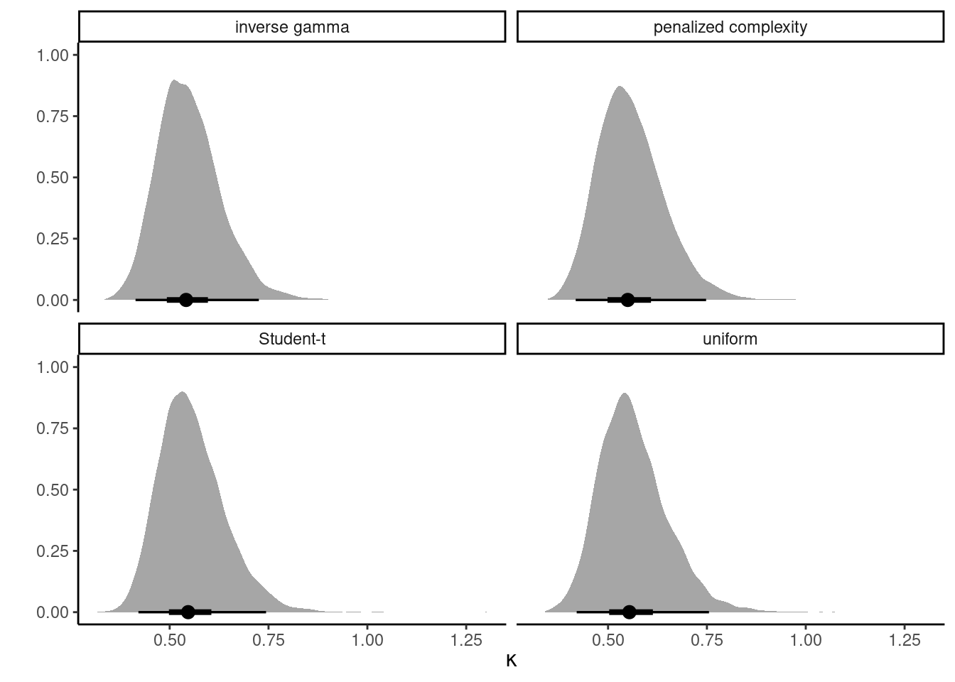
Figure 4: Posterior density of $τ$ for four different priors. The circle denotes the median and the bars the 50% and 95% percentile credible intervals.

Basically indistinguishable results for the random scale..

Eight schools example

Average results on SAT program, for eight schools (Rubin, 1981).

The hierarchical model is

$\begin{aligned} Y_{i} & \sim Gauss (μ + η_{i}, σ_{i}^{2}) \\ μ & \sim Gauss (0, 100) \\ η_{i} & \sim Gauss (0, τ^{2}) \end{aligned}$ Given the large sample in each school, we treat $σ_{i}$ as fixed data by using the sample standard deviation.

Sensibility analysis for eight schools example

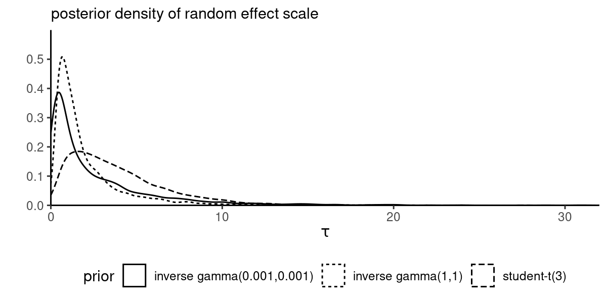
Figure 5: Posterior density of the school-specific random effects standard deviation $τ$ under different priors.

References

Brodeur, M., Ruer, P., Léger, P.-M., & Sénécal, S. (2021). Smartwatches are more distracting than mobile phones while driving: Results from an experimental study. Accident Analysis & Prevention, 149, 105846. https://doi.org/10.1016/j.aap.2020.105846

Gelman, A. (2006). Prior distributions for variance parameters in hierarchical models (comment on article by Browne and Draper). Bayesian Analysis, 1(3), 515–534. https://doi.org/10.1214/06-ba117a

Matias, J. N., Munger, K., Le Quere, M. A., & Ebersole, C. (2021). The Upworthy Research Archive, a time series of 32,487 experiments in U.S. media. Scientific Data, 8(195). https://doi.org/10.1038/s41597-021-00934-7

McElreath, R. (2020). Statistical rethinking: A Bayesian course with examples in R and STAN (2nd ed.). Chapman; Hall/CRC.

Rubin, D. B. (1981). Estimation in parallel randomized experiments. Journal of Educational Statistics, 6(4), 377–401. https://doi.org/10.3102/10769986006004377

Simpson, D., Rue, H., Riebler, A., Martins, T. G., & Sørbye, S. H. (2017). Penalising model component complexity: A principled, practical approach to constructing priors. Statistical Science, 32(1), 1–28. https://doi.org/10.1214/16-sts576