# Standard Gaussian truncated on [0,1]
candidate <- rnorm(1e5)
trunc_samp <- candidate[candidate >= 0 & candidate <= 1]
# Acceptance rate
length(trunc_samp)/1e5
[1] 0.34289[1] 0.3413447Monte Carlo methods, Markov chains and the Metropolis–Hastings algorithm
Last compiled Tuesday Apr 15, 2025
How to circumvent the problem of intractable posteriors?
We focus on Monte Carlo methods.
If \(F\) is an absolutely continuous distribution function, then \[F(X) \sim \mathsf{unif}(0,1).\] The inversion method consists in applying the quantile function \(F^{-1}\) to \(U \sim \mathsf{unif}(0,1)\), viz. \[F^{-1}(U) \sim X.\]
Consider a random variable \(Y\) with distribution function \(F\).
If \(X\) follows the same distribution as \(Y\), but restricted over the interval \([a,b]\), then \[\Pr(X \leq x) = \frac{F(x) - F(a)}{F(b)-F(a)}, \qquad a \leq x \leq b,\]
Therefore, \[F^{-1}[F(a) + \{F(b)-F(a)\}U] \sim X.\]
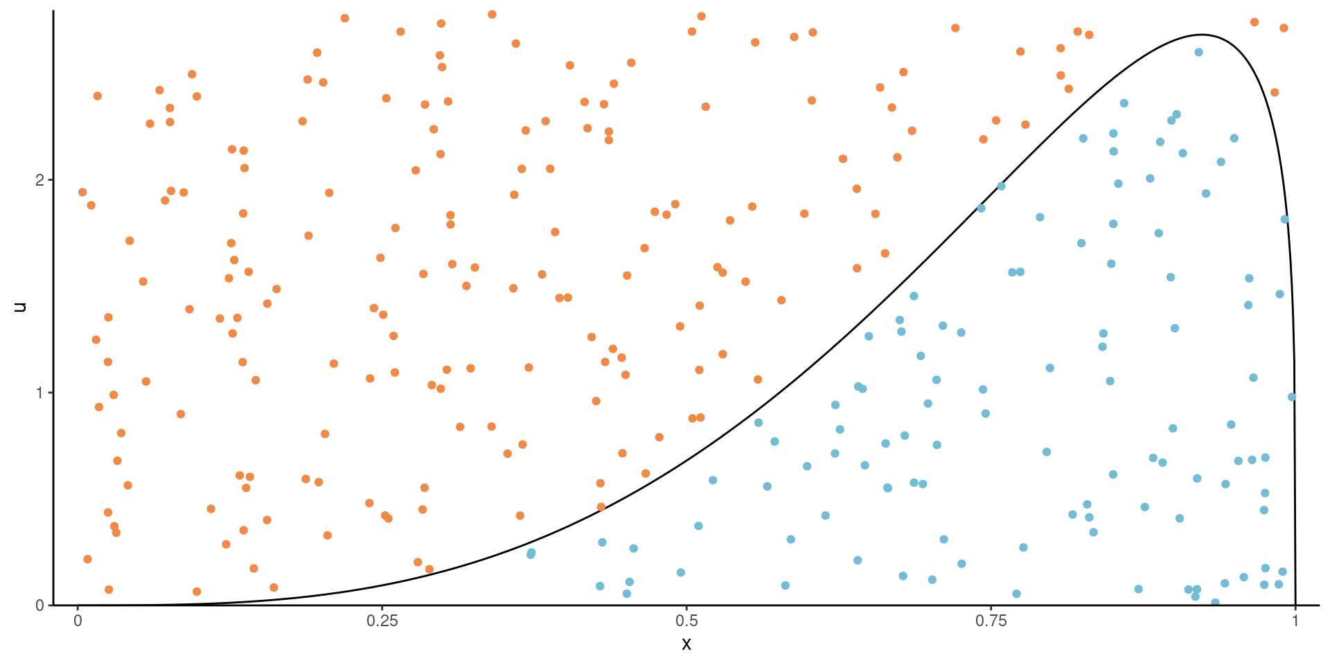
Consider a \(d\)-variate random vector \(\boldsymbol{X},\) independent of \(U \sim \mathsf{unif}(0,1)\) and \(c>0\). If \((\boldsymbol{X}, U)\) is uniformly distributed on the set \[\begin{align*} \mathcal{A}_{f}=\{(\boldsymbol{x}, u): 0 \leq u \leq c f(\boldsymbol{x})\}, \end{align*}\] then \(\boldsymbol{X}\) has density \(f(\boldsymbol{x}).\)
Figure 1: Illustration of the fundamental theorem of simulation. All points in blue below the density curve belong to \(\mathcal{A}_f.\)
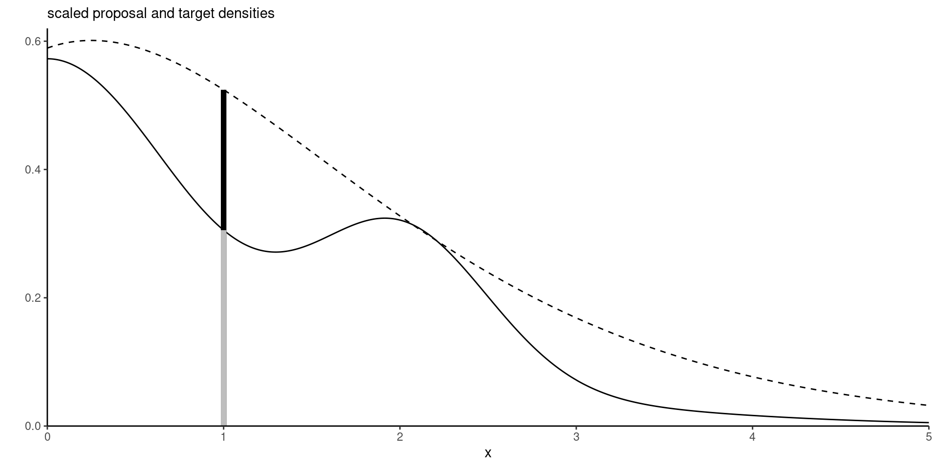
Figure 2: Target density (full) and scaled proposal density (dashed): the vertical segment at \(x=1\) shows the percentage of acceptance for a uniform slice under the scaled proposal, giving an acceptance ratio of 0.58.
Good choices must satisfy the following constraints:
Consider sampling \(Y \sim \mathsf{Gauss}(\mu, \sigma^2)\), but truncated in the interval \((a, b)\). The target density is \[\begin{align*} p(x; \mu, \sigma, a, b) = \frac{1}{\sigma}\frac{\phi\left(\frac{x-\mu}{\sigma}\right)}{\Phi(\beta)-\Phi(\alpha)}. \end{align*}\] for \(\alpha= (a-\mu)/\sigma\) and \(\beta = (b-\mu)/\sigma\). where \(\phi(\cdot), \Phi(\cdot)\) are respectively the density and distribution function of the standard Gaussian distribution.
The acceptance rate is \(C^{-1} = \{\Phi(\beta) - \Phi(\alpha)\}\)
Since the Gaussian is a location scale family, the inversion method gives \[\begin{align*} X \sim \mu + \sigma\Phi^{-1}\left[\Phi(\alpha) + \{\Phi(\beta)-\Phi(\alpha)\}U\right] \end{align*}\]
We however need to evaluate \(\Phi\) numerically (no closed-form expression).
The method fails for rare event simulation because the computer returns
implying that \(a \leq 8.3\) for this approach to work (Botev & L’Écuyer, 2017).
We consider simulation from a standard Gaussian truncated above \(a>0\)
Write the density of the truncated Gaussian as (Devroye, 1986, p. 381)\[f(x) = \frac{\exp(-x^2/2)}{\int_{a}^{\infty}\exp(-z^2/2)\mathrm{d} z} =\frac{\exp(-x^2/2)}{c_1}.\]
Note that, for \(x \geq a\), \[c_1f(x) \leq \frac{x}{a}\exp\left(-\frac{x^2}{2}\right)= a^{-1}\exp\left(-\frac{a^2}{2}\right)g(x);\] where \(g(x)\) is the density of a Rayleigh variable shifted by \(a\).
The constant \(C= \exp(-a^2/2)(c_1a)^{-1}\) approaches 1 quickly as \(a \to \infty\) (asymptotically optimality).
The shifted Rayleigh has distribution function \[G(x) = 1-\exp\{(a^2-x^2)/2\}, x \geq a.\]
Marsaglia algorithm
For sampling on \([a,b]\) with \(a\) very large, propose from a Rayleigh truncated above at \(b\) (Botev & L’Écuyer, 2017).
Plain ordinary Monte Carlo is great, but few algorithms are generic enough to be useful in complex high-dimensional problems.
We will instead typically build Markov chains that target an invariant stationary distribution.
Markov chain Monte Carlo methods generate correlated draws.
Questions:
We need to do a little theoretical detour to answer these questions.
A stochastic process is
Strong stationarity implies weak stationarity.
Consider a first-order autoregressive process, or \(\mathsf{AR}(1)\),
\[Y_t = \mu + \phi(Y_{t-1} - \mu) + \varepsilon_t,\] where
If \(|\phi| < 1\), the process is stationary, otherwise the variance increases with \(t\).
If the process is weakly stationary, then \(\mathsf{E}_{Y_{t}}(Y_t)=\mathsf{E}_{Y_{t-1}}(Y_{t-1})\) \[\begin{align*} \mathsf{E}_{Y_{t}}(Y_t) &= \mathsf{E}_{Y_{t-1}}\left\{\mathsf{E}_{Y_{t} \mid Y_{t-1}}(Y_t)\right\} \\&= \mu(1-\phi) + \phi\mathsf{E}_{Y_{t-1}}(Y_{t-1}) \end{align*}\] and so the unconditional mean is \(\mu\). For the variance, we have \[\begin{align*} \mathsf{Va}_{Y_{t}}(Y_t) &= \mathsf{E}_{Y_{t-1}}\left\{\mathsf{Va}_{Y_{t} \mid Y_{t-1}}(Y_t)\right\} + \mathsf{Va}_{Y_{t-1}}\left\{\mathsf{E}_{Y_{t} \mid Y_{t-1}}(Y_t)\right\}\\ & = \sigma^2 + \mathsf{Va}_{Y_{t-1}}\left\{\mu + \phi(Y_{t-1} - \mu)\right\} \\&= \sigma^2 + \phi^2 \mathsf{Va}_{Y_{t-1}}(Y_{t-1}). \end{align*}\] and the unconditional variance is \(\mathsf{Va}_{Y_t}(Y_t) = \sigma^2/(1-\phi^2).\)
The covariance at lag \(k\), in terms of innovations, gives \[\begin{align*} \gamma_k = \mathsf{Co}(Y_t, Y_{t-k}) = \mathsf{Va}(\phi Y_{t-1}, Y_{t-k}) + \mathsf{Va}(\varepsilon_t, Y_{t-k}) = \phi \gamma_{k-1} \end{align*}\] since \(\varepsilon_t\) is independent of the past. We thus find \[\gamma_k = \phi^k\mathsf{Va}(Y_t).\]
The \(\mathsf{AR}(1)\) process is first-order Markov since the conditional distribution \(p(Y_t \mid Y_{t-1}, \ldots, Y_{t-p})\) equals \(p(Y_t \mid Y_{t-1}).\)
Intuitively, a sample of correlated observations carries less information than an independent sample of draws.
The variance of the sample average is \[\begin{align*} \mathsf{Va}\left(\overline{Y}_T\right) &= \frac{1}{T^2}\sum_{t=1}^T \sum_{s=1}^T \mathsf{Co}(Y_t, Y_s) \\&= \frac{1}{T^2}\sum_{t=1}^T \mathsf{Va}(Y_t) + \frac{2}{T^2} \sum_{t=1}^{T-1}\sum_{s = t+1}^T \mathsf{Co}(Y_t, Y_s). \end{align*}\] Under independence and assuming stationarity, we get \(\mathsf{Va}\left(\overline{Y}_T\right)=\sigma^2/T.\)
If the second moments are finite, the scaled limiting variance of the sample mean simplifies to \[\begin{align*} \lim_{T \to \infty} T\mathsf{Va}\left(\overline{Y}_T\right) = \tau^2 \left\{1+2\sum_{t=1}^\infty \rho_t\right\}. \end{align*}\] which is a function of
The effective sample size is, loosely speaking, the equivalent number of observations if the \(B\) marginal posterior draws where independent and more formally \[ \mathsf{ESS} = \frac{B}{\left\{1+2\sum_{t=1}^\infty \rho_t\right\}} \] where \(\rho_t\) is the lag \(t\) correlation.
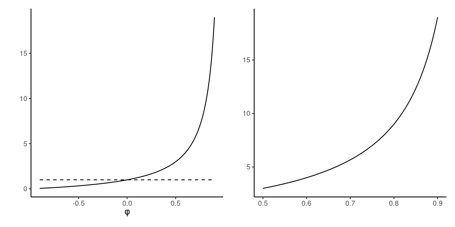
The lag-\(k\) correlation of the stationary autoregressive process of order 1 is \(\phi^k\), so \[1+2\sum_{t=1}^\infty \rho_t = 1 + 2 \left(\frac{1}{1-\phi}-1\right) = \frac{1+\phi}{1-\phi}.\]
Figure 3: Left: scaled asymptotic variance of the sample mean for AR(1) (full line) and independent observations with unit marginal variance (dashed). Right: variance ratio for positive correlations for selected range.
To get the same precision for the mean of \(\mathsf{AR}(1)\) process with \(\phi \approx 0.75\) than with i.i.d. data, we would need 7 times as many observations.
The price to pay for having correlated samples is
inefficiency
The higher the autocorrelation, the larger the variability of our estimators.
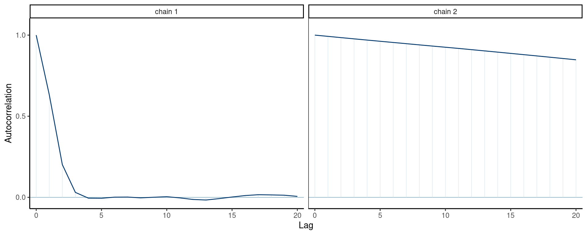
We can look at the autocorrelation function to check the efficiency.
Figure 4: Correlogram of two Markov chains. These plots, often called acf or autocorrelation functions, show the lag-k sample autocorrelation against lag number.
If a Markov chain is irreducible and acyclic, it has a unique stationary distribution.
Consider discrete Markov chains over the integers \(1, 2, 3\) with transition matrices
\[ P_1 = \begin{pmatrix} 0.5 & 0.3 & 0.2 \\ 0 & 0.4 & 0.6 \\ 0 & 0.5 & 0.5 \end{pmatrix}, \quad P_2 = \begin{pmatrix} 0 & 0 & 1 \\ 1 & 0 & 0 \\ 0 & 1 & 0 \end{pmatrix}. \] Chain 1 is reducible to \(\{2, 3\}\), chain 2 is cyclical.
Ergodicity means that two segments of a time series far enough apart act as independent.
Let \(\{Y_t\}\) is a weakly stationary sequence with mean \(\mathsf{E}(Y_t)=\mu\) and \(\gamma_h = \mathsf{Cov}(Y_t, Y_{t+h})\). Then, if the autocovariance series is convergent, meaning \[\sum_{t=0}^\infty |\gamma_h| < \infty,\] then \(\{Y_t\}\) is ergodic for the mean and \(\overline{Y} \stackrel{\mathrm{p}}{\to} \mu\).
The ergodic theorem is a law of large numbers for stochastic processes that allows for serial dependence between observations, provided the latter is not too large.
Any transformation \(g(\cdot)\) of a stationary and ergodic process \(\{Y_t\}\) retains the properties, so \(\overline{g} = T^{-1} \sum_{t=1}^T g(Y_t) \to \mathsf{E}\{g(Y_t)\}\) as \(T \to \infty.\)
The ergodic theorem holds even if the chain is cyclical.
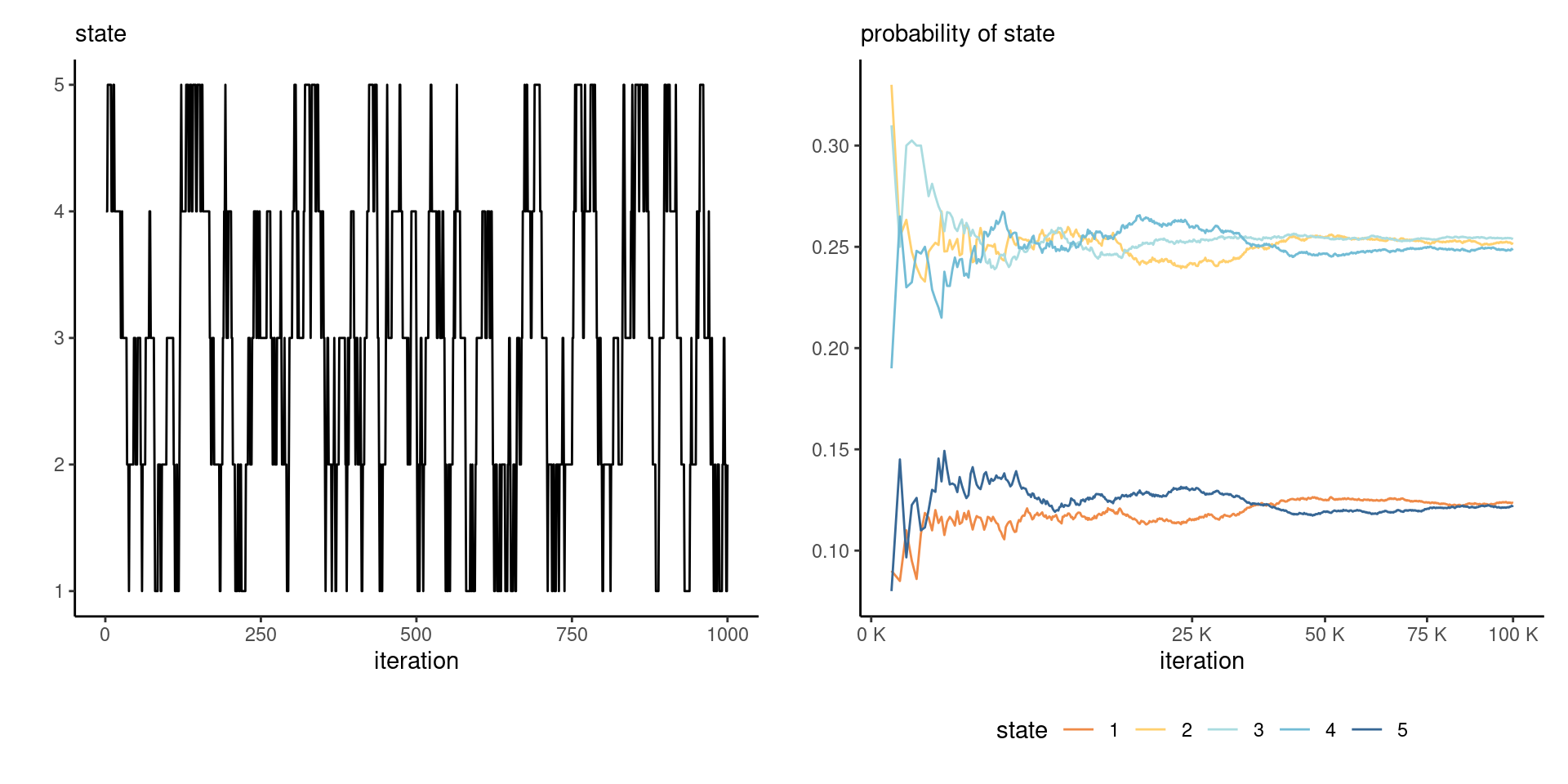
Consider a transition \(P\) on \(1, \ldots, 5\) defined as \[ P = \begin{pmatrix} \frac{2}{3} & \frac{1}{3} & 0 & 0 & 0 \\ \frac{1}{6} & \frac{2}{3} & \frac{1}{6} & 0 & 0 \\ 0 & \frac{1}{6} & \frac{2}{3} & \frac{1}{6} & 0 \\ 0 & 0 & \frac{1}{6} & \frac{2}{3} & \frac{1}{6} \\ 0 & 0 & 0 & \frac{1}{3} & \frac{2}{3} \\ \end{pmatrix} \] The stationary distribution is the value of the row vector \(\boldsymbol{p},\) such that \(\boldsymbol{p} = \boldsymbol{p}\mathbf{P}\) for transition matrix \(\mathbf{P}\): we get \(\boldsymbol{p}=(1,2,2,2,1)/8.\)
Figure 5: Discrete Markov chain on integers from 1 to 5, with traceplot of 1000 first iterations (left) and running mean plots of sample proportion of each state visited (right).
We consider simulating from a distribution with associated density function proportional to \(p(\cdot)\)
We use a conditional density \(q(\boldsymbol{\theta} \mid \boldsymbol{\theta}^{\text{cur}})\) to generate proposals from the current value \(\boldsymbol{\theta}^{\text{cur}}.\)
Starting from an initial value \(\boldsymbol{\theta}_0\): for \(t=1, \ldots, T\)
The Metropolis–Hastings algorithm satisfies a technical condition (detailed balance) that ensures that the Markov chain generated is reversible.
If the proposal is symmetric, the ratio of proposal densities is \[q(\boldsymbol{\theta}_{t-1} \mid \boldsymbol{\theta}_t^{\star} ) / q(\boldsymbol{\theta}_t^{\star} \mid \boldsymbol{\theta}_{t-1}) = 1.\]
Common examples include random walk proposals \[\boldsymbol{\theta}_t^{\star} \gets \boldsymbol{\theta}_{t-1} + \tau Z,\] where \(Z \sim \mathsf{Gauss}(0,1).\)
If we pick instead a global proposal, we must ensure that \(q\) samples in far regions (recall rejection sampling), otherwise …
Good proposals include heavy tailed distribution such as Student-\(t\) with small degrees of freedom,
centered at the maximum a posteriori \(\widehat{\boldsymbol{\theta}}\) and
with scale matrix proportional to \(-\mathbf{H}^{-1}(\boldsymbol{\theta}_t^{\star})\), where \(\mathbf{H}(\cdot)\) is the Hessian of the (unnormalized) log posterior.
We model the Poisson rates for headlines with questions or not. Our model is \[\begin{align*} Y_{i} &\sim \mathsf{Poisson}(n_i\lambda_i), \qquad (i=1,2)\\ \lambda_1 &= \exp(\beta + \kappa) \\ \lambda_2 &= \exp(\beta) \\ \beta & \sim \mathsf{Gauss}(\log 0.01, 1.5) \\ \kappa &\sim \mathsf{Gauss}(0, 1) \end{align*}\]
In regression models, scale inputs if possible.
data(upworthy_question, package = "hecbayes")
# Compute sufficient statistics
data <- upworthy_question |>
  dplyr::group_by(question) |>
  dplyr::summarize(ntot = sum(impressions),
                   y = sum(clicks))
# Create containers for MCMC
niter <- 1e4L
chain <- matrix(0, nrow = niter, ncol = 2L)
colnames(chain) <- c("beta","kappa")Perform all calculations on the log scale to avoid numerical overflow!
# Code log posterior as sum of log likelihood and log prior
loglik <- function(par, counts = data$y, offset = data$ntot, ...){
  lambda <- exp(c(par[1] + log(offset[1]), par[1] + par[2] + log(offset[2])))
 sum(dpois(x = counts, lambda = lambda, log = TRUE))
}
# Note common signature of function
logprior <- function(par, ...){
  dnorm(x = par[1], mean = log(0.01), sd = 1.5, log = TRUE) +
    dnorm(x = par[2], log = TRUE)
}
logpost <- function(par, ...){
  loglik(par, ...) + logprior(par, ...)
}Use good starting values for your Markov chains, such as maximum a posteriori.
# Compute maximum a posteriori (MAP)
map <- optim(
  par = c(-4, 0.07),
  fn = logpost,
  control = list(fnscale = -1),
  offset = data$ntot,
  counts = data$y,
  hessian = TRUE)
# Use MAP as starting value
cur <- map$par
# Compute logpost_cur - we can keep track of this to reduce calculations
logpost_cur <- logpost(cur)
# Proposal covariance
cov_map <- -2*solve(map$hessian)
chol <- chol(cov_map)Use seed for reproducibility, do not compute posterior twice, compute log of acceptance ratio.
set.seed(80601)
naccept <- 0L
for(i in seq_len(niter)){
  # Multivariate normal proposal - symmetric random walk
  prop <- c(rnorm(n = 2) %*% chol + cur)
  logpost_prop <- logpost(prop)
  logR <- logpost_prop - logpost_cur
  if(logR > -rexp(1)){
    cur <- prop
    logpost_cur <- logpost_prop
    naccept <- naccept + 1L
  }
  chain[i,] <- cur
}1. Empirical mean and standard deviation for each variable,
plus standard error of the mean:
Mean SD Naive SE Time-series SE
beta -4.51268 0.001697 1.697e-05 6.176e-05
kappa 0.07075 0.002033 2.033e-05 9.741e-05
2. Quantiles for each variable:
2.5% 25% 50% 75% 97.5%
beta -4.51591 -4.51385 -4.51273 -4.51154 -4.50929
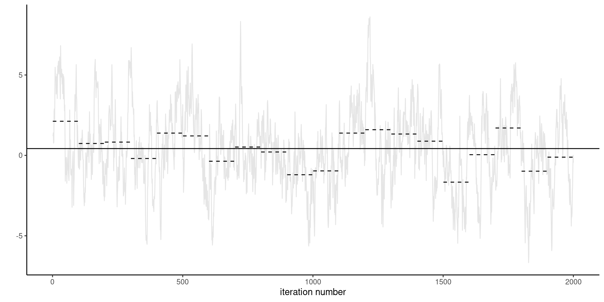
kappa 0.06673 0.06933 0.07077 0.07212 0.07463Geyer (2011) recommends to segment the time series into batches
Figure 6: Calculation of the standard error of the posterior mean using the batch method.
We can also fit an high-order autoregressive process \(\mathsf{AR}(p)\) and approximate the unconditional variance by that, and divide by \(\sqrt{T}\).
![]()