Visualisation avec ggplot2

# Visualisation<br>avec `ggplot2`

.class-info[
<figure>
  <img src="img/03/ggplot-logo.png" alt="ggplot" title="ggplot" width="15%">
</figure>
]

<br>

---

# Voitures et cylindrée

.box-inv-1.medium[Quelle est la relation entre la cylindrée d'une voiture <br>et son autonomie?
]

---

# À votre tour #1

```r
library(ggplot2)
ggplot(data = mpg) +
  geom_point(mapping = aes(x = displ, 
                           y = hwy))
```

---

```r
ggplot(data = mpg) +
  geom_point(mapping = aes(x = displ, 
                           y = hwy))
```

---

# La grammaire des graphiques

.pull-left.center[

]

.box-inv-1.medium[Composante esthétique]

.box-1.sp-after[Position, forme, couleur, etc.]

.box-inv-1.medium[Variables]

]

# Les voitures avec une plus grande cylindrée parcourent plus de distance?

---

# Esthétique

.box-inv-1.small[`color` (discrète)]

.box-inv-1.small[`color` (continue)]

<img src="MATH60602-diapos2c-visualisation_files/figure-html/aes-color-continuous-1.png" width="100%" style="display: block; margin: auto;" />
]

.box-inv-1.small[`size`]

.box-inv-1.small[`fill`]

<img src="MATH60602-diapos2c-visualisation_files/figure-html/aes-fill-1.png" width="100%" style="display: block; margin: auto;" />
]

.box-inv-1.small[`shape`]

.box-inv-1.small[`alpha`]

<img src="MATH60602-diapos2c-visualisation_files/figure-html/aes-alpha-1.png" width="100%" style="display: block; margin: auto;" />
]

---

# Associer colonnes et esthétiques

```r
ggplot(mpg) + geom_point(aes(x = displ, y = hwy, color = class))
ggplot(mpg) + geom_point(aes(x = displ, y = hwy, size = class))
ggplot(mpg) + geom_point(aes(x = displ, y = hwy, shape = class))
ggplot(mpg) + geom_point(aes(x = displ, y = hwy, alpha = class))
```
]

---

```r
ggplot(data = mpg) +
  geom_point(mapping = aes(x = displ, y = hwy, color = class))
```

---

# À votre tour #2

.box-1[Y a-t-il des différences selon qu'on associe une composante esthétique à des variables discrètes ou continues?]

---

# Comment créer ce graphique?

---

```r
ggplot(mpg) +
  geom_point(aes(x = displ, 
                 y = hwy, 
                 color = class))
```
]

---

```r
ggplot(mpg) +
  geom_point(aes(x = displ, 
                 y = hwy), 
             color = "blue")
```
]

---

```r
ggplot(mpg) +
  geom_point(aes(x = displ, 
                 y = hwy, 
                 color = "blue"))
```

<img src="MATH60602-diapos2c-visualisation_files/figure-html/unnamed-chunk-8-1.png" width="100%" style="display: block; margin: auto;" />
]
]

```r
ggplot(mpg) +
  geom_point(aes(x = displ, 
                 y = hwy), 
             color = "blue")
```

<img src="MATH60602-diapos2c-visualisation_files/figure-html/unnamed-chunk-9-1.png" width="100%" style="display: block; margin: auto;" />
]
]

---

---

# Similarités et différences?

.pull-left[
<img src="MATH60602-diapos2c-visualisation_files/figure-html/unnamed-chunk-10-1.png" width="100%" style="display: block; margin: auto;" />
]

.pull-right[
<img src="MATH60602-diapos2c-visualisation_files/figure-html/unnamed-chunk-11-1.png" width="100%" style="display: block; margin: auto;" />
]

---

# Géométries

<code class ='r hljs remark-code'>ggplot(data = <b><span style="background-color:#CBB5FF">DONNÉES</span></b>) +<br>&nbsp;&nbsp;<b><span style="background-color:#FFDFD1">FONCTION_GEOM</span></b>(mapping = aes(APPLICATION: VARIABLES > COMPOSANTESESTHÉTIQUE ))</code>

---

# Géométries

<table>
  <tr>
    <th class="cell-left"></th>
    <th class="cell-left">Exemple de géométrie</th>
    <th class="cell-left">Sortie</th>
  </tr>
  <tr>
    <td class="cell-left"><img src="img/03/geom_bar.png"></td>
    <td class="cell-left"><code class="remark-inline-code">geom_bar()</code></td>
    <td class="cell-left">Diagramme à bande</td>
  </tr>
  <tr>
    <td class="cell-left"><img src="img/03/geom_text.png"></td>
    <td class="cell-left"><code class="remark-inline-code">geom_text()</code></td>
    <td class="cell-left">Texte</td>
  </tr>
  <tr>
    <td class="cell-left"><img src="img/03/geom_point.png"></td>
    <td class="cell-left"><code class="remark-inline-code">geom_point()</code></td>
    <td class="cell-left">Nuage de points</td>
  </tr>
  <tr>
    <td class="cell-left"><img src="img/03/geom_boxplot.png"></td>
    <td class="cell-left"><code class="remark-inline-code">geom_boxplot()</code>&emsp;</td>
    <td class="cell-left">Boîte à moustaches</td>
  </tr>
</table>

---

# Inventaire de géométries

.box-1[Voir [la documentation `ggplot2`](https://ggplot2.tidyverse.org/reference/index.html#section-layer-geoms) pour<br>un exemple exhaustif avec toutes les géométries.]

---

# À votre tour #3

.pull-left[
<img src="MATH60602-diapos2c-visualisation_files/figure-html/unnamed-chunk-12-1.png" width="100%" style="display: block; margin: auto;" />
]

.pull-right[
<img src="MATH60602-diapos2c-visualisation_files/figure-html/unnamed-chunk-13-1.png" width="100%" style="display: block; margin: auto;" />
]

---

# À votre tour #4

.box-1[Produisez un histogramme de `hwy`. Utilisez l'aide mémoire.<br>Indice: ne pas fournir de variable `y`.]

---

# À votre tour #5

.box-1[Colorez la densité de `hwy` par `class`.<br>Utilisez l'aide mémoire.<br> Indice: ne pas fournir de variable `y`.]

---

# Graphiques complexes!

---

# À votre tour #6

```r
ggplot(data = mpg) +
  geom_point(mapping = aes(x = displ, y = hwy)) +
  geom_smooth(mapping = aes(x = displ, y = hwy))
```

---

# Global vs. local

.box-inv-1[Toute composante esthétique dans `ggplot()`<br> est utilisée dans toutes les strates `geom_`]

```r
ggplot(data = mpg, mapping = aes(x = displ, y = hwy)) +
  geom_point() +
  geom_smooth()
```

<img src="MATH60602-diapos2c-visualisation_files/figure-html/unnamed-chunk-20-1.png" width="60%" style="display: block; margin: auto;" />
]

---

# Global vs. local

.box-inv-1[Toute composante esthétique fournie dans la strate `geom_`<br> s'applique uniquement à cette dernière]

```r
ggplot(data = mpg, mapping = aes(x = displ, y = hwy)) +
  geom_point(mapping = aes(color = drv)) +
  geom_smooth()
```

<img src="MATH60602-diapos2c-visualisation_files/figure-html/unnamed-chunk-21-1.png" width="60%" style="display: block; margin: auto;" />
]

---

---

# Bien plus

---

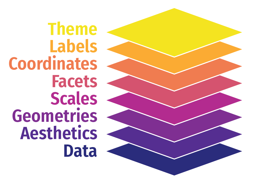# Mettre tout ensemble

.box-inv-1.medium[On construit le graphique étape par étape<br>pour voir l'impact des strates<br>sur l'apparence.]

---

```r
*ggplot(data = mpg,
*      mapping = aes(x = displ,
*                    y = hwy,
*                    color = drv))
```
]

---

```r
ggplot(data = mpg,
       mapping = aes(x = displ,
                     y = hwy,
                     color = drv)) +
* geom_point()
```
]

---

```r
ggplot(data = mpg,
       mapping = aes(x = displ,
                     y = hwy,
                     color = drv)) +
  geom_point() +
* geom_smooth()
```
]

---

```r
ggplot(data = mpg,
       mapping = aes(x = displ,
                     y = hwy,
                     color = drv)) +
  geom_point() +
* geom_smooth(method = "lm")
```
]

---

```r
ggplot(data = mpg,
       mapping = aes(x = displ,
                     y = hwy,
                     color = drv)) +
  geom_point() +
  geom_smooth(method = "lm") +
* scale_color_viridis_d()
```
]

---

```r
ggplot(data = mpg,
       mapping = aes(x = displ,
                     y = hwy,
                     color = drv)) +
  geom_point() +
  geom_smooth(method = "lm") +
  scale_color_viridis_d() +
* facet_wrap(vars(drv), ncol = 1)
```
]

---

```r
ggplot(data = mpg,
       mapping = aes(x = displ,
                     y = hwy,
                     color = drv)) +
  geom_point() +
  geom_smooth(method = "lm") +
  scale_color_viridis_d() +
  facet_wrap(vars(drv), ncol = 1) +
*   labs(x = "cylindrée (litres)",
*      y = "",
*      subtitle = "autonomie sur l'autoroute (mile au gallon)",
*      color = "type",
*      title = "Cylindrée imposante rime avec moins d'autonomie.",
*      caption = "Je connais rien aux voitures")
```
]

---

```r
ggplot(data = mpg,
       mapping = aes(x = displ,
                     y = hwy,
                     color = drv)) +
  geom_point() +
  geom_smooth(method = "lm") +
  scale_color_viridis_d() +
  facet_wrap(vars(drv), ncol = 1) +
  labs(x = "cylindrée (litres)", 
       y = "",
       subtitle = "autonomie sur l'autoroute (mile au gallon)",
       color = "type", 
       title = "Cylindrée imposante rime avec moins d'autonomie.",
       caption = "Je connais rien aux voitures") +
* theme_bw()
```
]

---

```r
ggplot(data = mpg, 
       mapping = aes(x = displ,
                     y = hwy,
                     color = drv)) +
  geom_point() +
  geom_smooth(method = "lm") +
  scale_color_viridis_d() +
  facet_wrap(vars(drv), ncol = 1) +
  labs(x = "cylindrée (litres)", 
       y = "",
       subtitle = "autonomie sur l'autoroute (mile au gallon)",
       color = "type", 
       title = "Cylindrée imposante rime avec moins d'autonomie.",
       caption = "Je connais rien aux voitures") +
  theme_bw() +
* theme(legend.position = "bottom")
```
]

---

```r
ggplot(data = mpg, 
       mapping = aes(x = displ,
                     y = hwy,
                     color = drv)) +
  geom_point() +
  geom_smooth(method = "lm") + 
  scale_color_viridis_d() +
  facet_wrap(vars(drv), ncol = 1) +
  labs(x = "cylindrée (litres)", 
       y = "",
       subtitle = "autonomie sur l'autoroute (mile au gallon)",
       color = "type", 
       title = "Cylindrée imposante rime avec moins d'autonomie.",
       caption = "Je connais rien aux voitures") +
  theme_bw() +
  theme(legend.position = "bottom")
```
]