The linear model equation is \[\boldsymbol{Y} = \underset{\text{mean } \boldsymbol{\mu}}{\mathbf{X}\boldsymbol{\beta}} + \underset{\text{errors}}{\vphantom{\beta}\boldsymbol{\varepsilon}}\] and assume that \(\mathsf{E}(\boldsymbol{\varepsilon} \mid \mathbf{X})= \boldsymbol{0}_n\) and \(\mathsf{Va}(\boldsymbol{\varepsilon} \mid \mathbf{X}) = \sigma^2\mathbf{I}_n\).
The fitted model gives the decomposition \[\begin{align*}
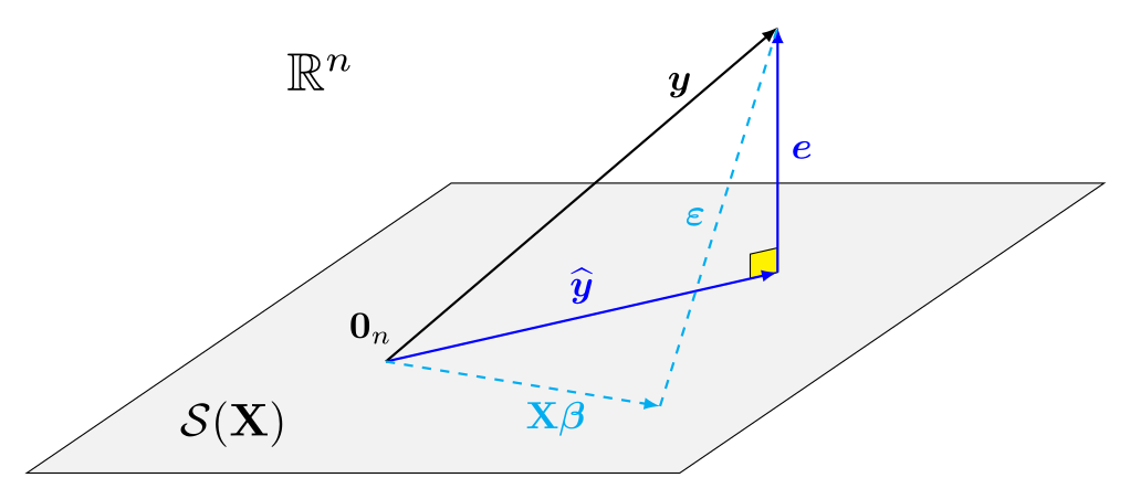
\underset{\text{observations}}{\boldsymbol{y}} = \underset{\text{fitted values}}{\widehat{\boldsymbol{y}}} + \underset{\text{residuals}}{\vphantom{y}\boldsymbol{e}}
\end{align*}\]
Projection matrices
For an \(n\times (p+1)\) matrix, the column space of \(\mathbf{X}\) is \[\begin{align*}
\mathcal{S}(\mathbf{X}) =\{\mathbf{X}\boldsymbol{a}, \boldsymbol{a} \in \mathbb{R}^{p+1}\}
\end{align*}\]
We can write the fitted values as the projection the observed response vector \(\boldsymbol{y}\) onto the linear span of the model matrix \(\mathbf{X}\), \[\begin{align*}
\underset{\text{fitted values}}{\widehat{\boldsymbol{y}}} = \underset{\substack{\text{model matrix $\times$}\\\text{OLS estimator}}}{\mathbf{X} \widehat{\boldsymbol{\beta}}} = \underset{\text{projection matrix}}{\mathbf{X}(\mathbf{X}^\top\mathbf{X})^{-1}\mathbf{X}^\top}\boldsymbol{y} = \mathbf{H}_{\mathbf{X}}\boldsymbol{y}
\end{align*}\] where \(\mathbf{H}_{\mathbf{X}} = \mathbf{X}(\mathbf{X}^\top\mathbf{X})^{-1}\mathbf{X}^\top\) is an \(n \times n\) orthogonal projection matrix.
\(\mathbf{H}_{\mathbf{X}}\) is a symmetric \(n \times n\) square matrix of rank \(p+1\).
An orthogonal projection matrix satisfies \(\mathbf{H}_{\mathbf{X}}\mathbf{H}_{\mathbf{X}} = \mathbf{H}_{\mathbf{X}}\) and \(\mathbf{H}_{\mathbf{X}} = \mathbf{H}_{\mathbf{X}}^\top\).
Visual depiction of the geometry
Consequences of orthogonality
The geometric representation has deep implications for inference that are useful for model diagnostics.
The fitted values \(\widehat{\boldsymbol{y}}\) and \(\boldsymbol{e}\) are uncorrelated
Idem for any column of \(\mathbf{X}\), since \(\mathbf{X}^\top\boldsymbol{e}=\boldsymbol{0}_{p+1}\).
Assuming \(\mathbf{1}_n \in \mathcal{S}(\mathbf{X})\) (e.g., the intercept is included in \(\mathbf{X}\)), the sample mean of \(\boldsymbol{e}\) is zero.
data(college, package ="hecstatmod")mod <-lm(salary ~ sex + field + rank + service, data = college)# Zero correlationscor(resid(mod), model.matrix(mod))[-1]## [1] -4.9e-17 -1.6e-17 3.7e-18 2.9e-18 1.3e-17cor(resid(mod), fitted(mod))## [1] -2.7e-17# Mean zero errorsmean(resid(mod))## [1] 1.5e-16
Graphical diagnostics
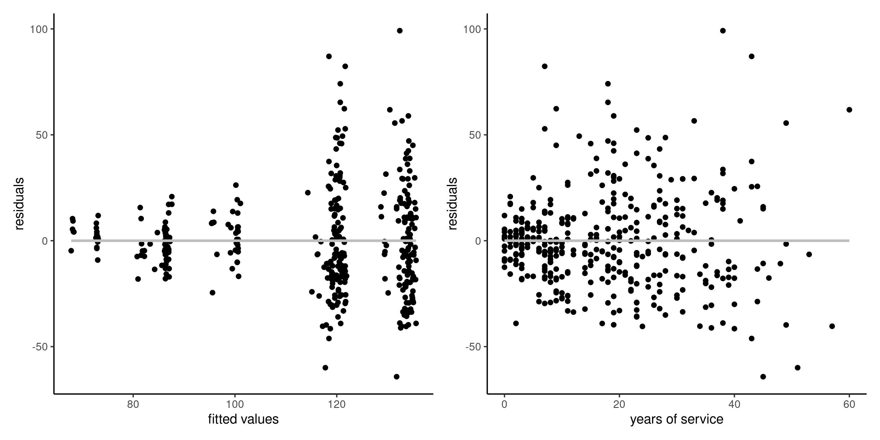
A linear regression of \(\widehat{\boldsymbol{y}}\) (or any column of \(\mathbf{X}\)) onto \(\boldsymbol{e}\) has zero intercept and slope.
Figure 1: Plot of residuals against fitted values (left), and against the explanatory variable service (right) for the linear regression of the college data. The intercept and the slope of the simple linear regressions are zero.
Residual patterns due to forgotten interactions, nonlinear terms, etc. could be picked up from pair plots of ordinary residuals against the explanatories.
Invariance
The fitted values \(\widehat{y}_i\) for two model matrices \(\mathbf{X}_a\) and \(\mathbf{X}_b\), are the same if they generate the same linear span, i.e., \(\mathcal{S}(\mathbf{X}_a) = \mathcal{S}(\mathbf{X}_b)\).
Since we define residuals as \[\boldsymbol{E}=(\mathbf{I}-\mathbf{H}_{\mathbf{X}})\mathbf{Y},\] it follows if \(Y_i \sim \mathsf{normal}(\mathbf{x}_i\boldsymbol{\beta}, \sigma^2)\) that
The marginal distribution of the errors is \(E_i \sim \mathsf{normal}\{0, \sigma^2(1-h_{ii})\}\).
The residuals are heteroscedastic, and their variance depends on the diagonal elements of the “hat matrix” \(\mathbf{H}_{\mathbf{X}}\), the collection \(\{h_{ii}\}\) for \((i=1, \ldots, n)\).
Since \(\mathbf{I}-\mathbf{H}_{\mathbf{X}}\) has rank \(n-p-1\), the residuals are linearly related (there are \(n-p-1\) free components).
We can show that \(\mathsf{Cov}(e_i, e_j) = -\sigma^2h_{ij}\): residuals are correlated.
Variance estimation and standardization
We want to standardize residuals to have mean zero and unit variance, but \(\sigma^2\) is unknown.
If we estimate \(\sigma^2\) by \(S^2\), we introduce additional dependence since \(S^2 = \sum_{i=1}^n e_i^2/(n-p-1)\), and \(e_i\) appears in the formula of the sample variance…
We consider estimation of the standard deviation \(S_{-i}\) by fitting the model to but the \(i\)th observation (jackknife estimator). Then, \(e_i\) is independent of \(S_{-i}\)
No need to refit the model! The formula can be written as \[S_{-i}^2= \frac{(n-p-1)S^2 - e_i^2/(1-h_{ii})}{n-p-2}.\]
Externally studentized residuals
Define the jackknife (or externally) studentized residuals as \[r_i = \frac{e_i}{S_{-i}(1-h_{ii})^{1/2}}.\]
In R, use rstudent to obtain the values.
The marginal distribution of \(R_i\) is \(\mathsf{Student}(n-p-2)\) for \(i=1, \ldots, n\).
But the collection \(R_1, \ldots, R_n\) are not independent.
Leverage
The diagonal elements of the hat matrix \(h_{ii} = \partial \widehat{y}_i/\partial y_i\) represent the leverage of an observation.
Leverage values tell us how much each point impacts the fit: they are strictly positive, are bounded below by \(1/n\) and above by \(1\).
The sum of the leverage values is \(\sum_{i=1}^n h_{ii}=p+1\): in a good design, each point has approximately the same contribution, with average weight \((p+1)/n\).
Points with high leverage are those that have unusual combinations of explanatories.
One condition for the OLS estimator \(\widehat{\boldsymbol{\beta}}\) to be consistent and asymptotically normal is that \(\max_{i=1}^n h_{ii} \to 0\) as \(n \to \infty\): no observation dominates the fit.
Influential observations vs outliers
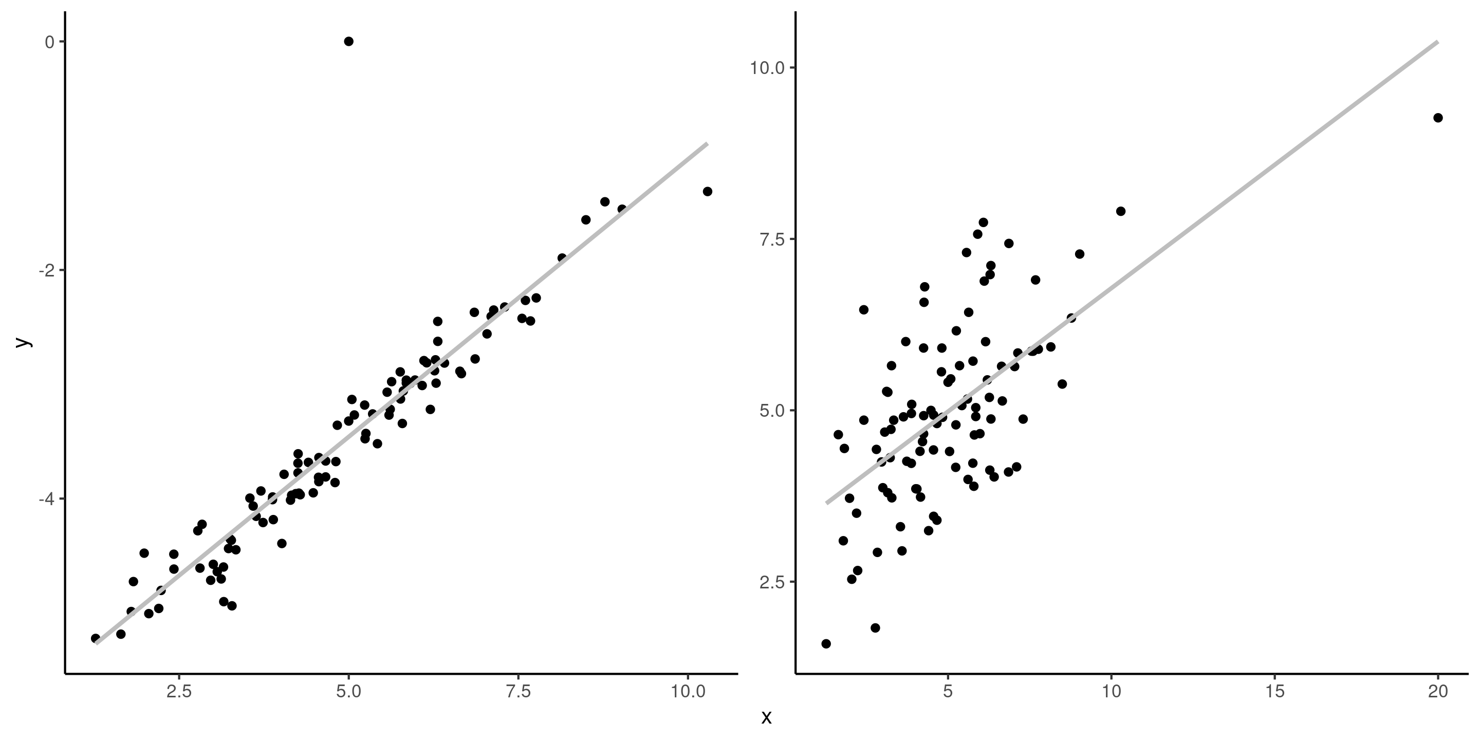
It is important to distinguish betwen influential observations (which have unusual \(\mathbf{x}\) value, i.e., far from the overall mean) and outliers (unusual value of the response \(y\)). If an observation is both an outlier and has a high leverage, it is problematic.
Figure 2: Outlier and influential observation. The left panel shows an outlier, whereas the right panel shows an influential variable (rightmost \(x\) value).
Cook distance
The Cook distance of an observation measures the standardized squared prediction error for data when we base the OLS estimator on all but the \(i\)th observation, say \(\widehat{\boldsymbol{\beta}}_{-i}\), and the predictions are \(\widehat{\boldsymbol{y}}_{-i}=\mathbf{X}\widehat{\boldsymbol{\beta}}_{-i}\).