The Pearson correlation coefficient quantifies the strength of the linear relationship between two random variables \(X\) and \(Y\). \[\begin{align*}
\rho= \mathsf{cor}(X, Y) = \frac{{\mathsf{Co}}(X,Y)}{\sqrt{{\mathsf{Va}}(X){\mathsf{Va}}(Y)}}.
\end{align*}\]
The sample correlation \(\rho \in [-1, 1]\).
\(|\rho|=1\) if and only if the \(n\) observations fall exactly on a line.
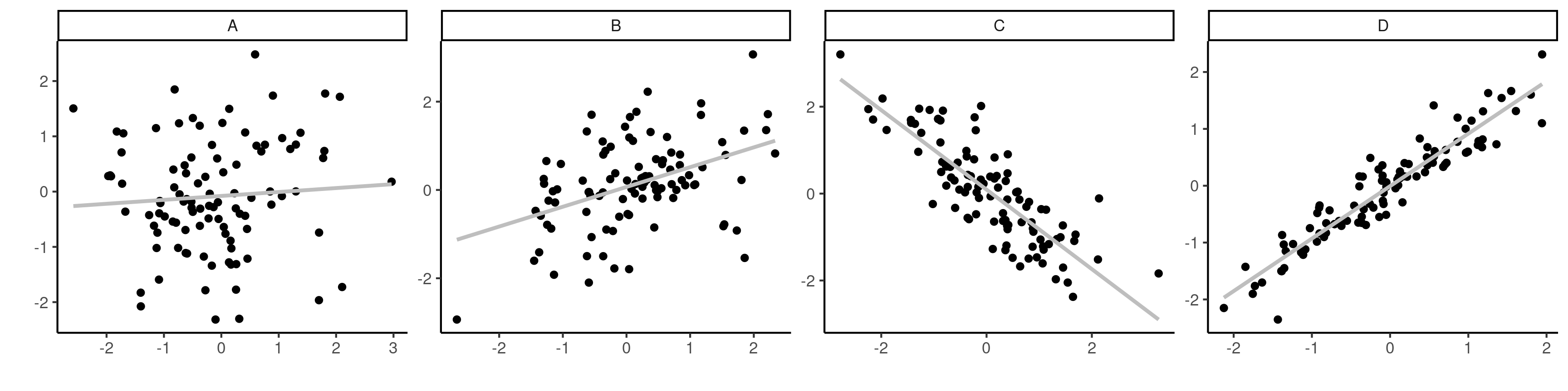
The larger \(|\rho|\), the less scattered the points are.
Properties of Pearson’s linear correlation coefficient
The sign determines the orientation of the slope.
If \(\rho>0\), the variables are positively associated, meaning \(Y\) increases on average with \(X\).
If \(\rho <0\), the association is negative and \(Y\) decreases on average with \(X\).
Figure 1: Scatterplots of observations with correlations of \(0.1\), \(0.5\), \(-0.75\) and \(0.95\) from \(A\) to \(D\).
Correlation and independence
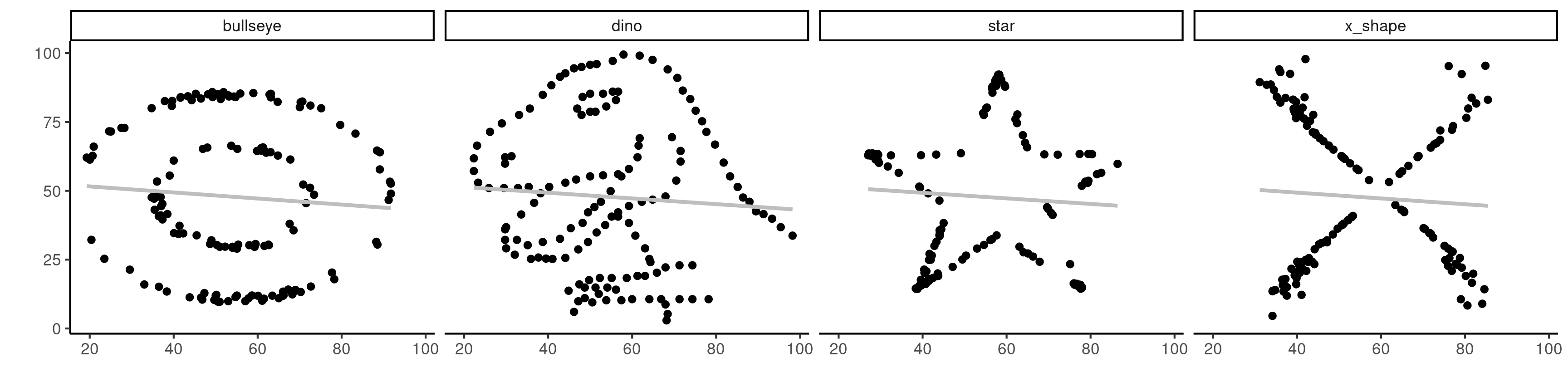
Independent variables are uncorrelated (not the other way around).
A correlation of zero only implies that there is no linear dependence between two variables.
Figure 2: Four datasets with dependent data having identical summary statistics and a linear correlation of -0.06.
Sum of squares decomposition
Suppose that we do not use any explanatory variable (i.e., the intercept-only model). In this case, the fitted value for \(Y\) is the overall mean and the sum of squared centered observations \[\begin{align*}
\mathsf{SS}_c=\sum_{i=1}^n (Y_i-\overline{Y})^2
\end{align*}\] where \(\overline{Y}\) represents the intercept-only fitted value.
When we include the \(p\) regressors, we get rather \[\begin{align*}
\mathsf{SS}_e=\sum_{i=1}^n (Y_i-\widehat{Y}_i)^2
\end{align*}\] The \(\mathsf{SS}_e\) is non-increasing when we include more variables.
Percentage of variance
Consider the sum of squared residuals for two models:
\(\mathsf{SS}_c\) is for the intercept-only model
\(\mathsf{SS}_e\) for the linear regression with model matrix \(\mathbf{X}\).
Consequently, \(\mathsf{SS}_c-\mathsf{SS}_e\) is the reduction of the error associated with including \(\mathbf{X}\) in the model \[\begin{align*}
R^2=\frac{\mathsf{SS}_c-\mathsf{SS}_e}{\mathsf{SS}_c}
\end{align*}\] This gives the proportion of the variability in \(\boldsymbol{Y}\) explained by \(\mathbf{X}\).
Coefficient of determination
We can show that the coefficient of determination is the square of Pearson’s linear correlation between the response \(\boldsymbol{y}\) and the fitted values \(\widehat{\boldsymbol{y}}\), \[R^2 = \mathsf{cor}^2(\boldsymbol{y}, \widehat{\boldsymbol{y}}).\]
data(college, package ="hecstatmod")mod <-lm(salary ~ sex + field + rank + service, data = college)summary(mod)$r.squared # R-squared from output## [1] 0.45y <- college$salary # response vectoryhat <-fitted(mod) # fitted valuecor(y, yhat)^2## [1] 0.45
\(R^2\) always takes a value between \(0\) and \(1\).
\(R^2\) is not a goodness-of-fit criterion: the coefficient is non-decreasing so the more explanatories are added to \(\mathbf{X}\), the higher the \(R^2\).