| lognuser | celcius | farenheit | rfarenheit |
|---|---|---|---|
| 7.36 | 1.5 | 34.7 | 35 |
| 8.06 | 0.2 | 32.4 | 32 |
| 8.67 | 6.8 | 44.2 | 44 |
| 8.58 | 10.1 | 50.2 | 50 |
| 8.70 | 10.3 | 50.5 | 51 |
Statistical modelling
06. Linear models (collinearity)
2024
Multicollinearity
- Multicollinearity describes when an explanatory variable (or several) is strongly correlated with a linear combination of other explanatory variables.
- One potential harm of multicollinearity is the decrease in precision: it increases the standard errors of the parameters.
Bixi and multicollinearity
We consider a simple illustration with temperature at 16:00 in Celcius and Farenheit (rounded to the nearest unit for \(\texttt{rfarenheit}\)) to explain log of daily counts of Bixi users for 2014–2019.
Linear invariance
Consider the log number of Bixi rentals per day as a function of the temperature in degrees Celcius and in Farenheit, rounded to the nearest unit. The postulated linear model is \[\begin{align*} \texttt{lognuser} = \beta_0 + \beta_{\texttt{c}} \texttt{celcius} + \beta_{\texttt{f}} \texttt{farenheit} + \varepsilon. \end{align*}\]
- The interpretation of \(\beta_{\texttt{c}}\) is “the average increase in number of rental per day when temperature increases by \(1{}^{\circ}\)C, keeping the temperature in Farenheit constant”…
- The two temperatures units are linearly related, \[1.8 \texttt{celcius} + 32 = \texttt{farenheit}.\]
Diving into the problem
Suppose that the true effect (fictional) effect of temperature on bike rental is \[\begin{align*} \mathsf{E}(\texttt{lognuser} \mid \cdot) = \alpha_0+ \alpha_1 \texttt{celcius}. \end{align*}\]
The coefficients for the model that only includes Farenheit are thus \[\begin{align*} \mathsf{E}(\texttt{lognuser} \mid \cdot)= \gamma_0 + \gamma_1\texttt{farenheit}, \end{align*}\] where \(\alpha_0 = \gamma_0 + 32\gamma_1\) and \(1.8\gamma_1 = \alpha_1\).
| Estimate | Std. Error | |
|---|---|---|
| (Intercept) | 8.844 | 0.028 |
| celcius | 0.049 | 0.001 |
| Estimate | Std. Error | |
|---|---|---|
| (Intercept) | 7.981 | 0.051 |
| farenheit | 0.027 | 0.001 |
Perfect collinearity
The parameters of the postulated linear model with both predictors, \[\begin{align*} \texttt{lognuser} = \beta_0 + \beta_{\texttt{c}} \texttt{celcius} + \beta_{\texttt{f}} \texttt{farenheit} + \varepsilon, \end{align*}\] are not identifiable, since any linear combination of the two solutions gives the same answer.
This is the same reason why we include \(K-1\) dummy variables for a categorical variable with \(K\) levels when the model already includes an intercept.
Lack of uniqueness of the solution
# Exact collinearity
linmod3_bixicoll  <- lm(lognuser ~ celcius + farenheit, data = bixicoll)
summary(linmod3_bixicoll)
##
## Call:
## lm(formula = lognuser ~ celcius + farenheit, data = bixicoll)
##
## Residuals:
##     Min      1Q  Median      3Q     Max
## -1.5539 -0.2136  0.0318  0.2400  0.8256
##
## Coefficients: (1 not defined because of singularities)
##             Estimate Std. Error t value Pr(>|t|)
## (Intercept)  8.84433    0.02819   313.7   <2e-16 ***
## celcius      0.04857    0.00135    35.9   <2e-16 ***
## farenheit         NA         NA      NA       NA
## ---
## Signif. codes:  0 '***' 0.001 '**' 0.01 '*' 0.05 '.' 0.1 ' ' 1
##
## Residual standard error: 0.354 on 1182 degrees of freedom
## Multiple R-squared:  0.522,  Adjusted R-squared:  0.521
## F-statistic: 1.29e+03 on 1 and 1182 DF,  p-value: <2e-16
Estimated coefficients with near-collinearity
# Approximate colinearity
linmod4_bixicoll  <- lm(lognuser ~ celcius + rfarenheit, data = bixicoll)
summary(linmod4_bixicoll)
##
## Call:
## lm(formula = lognuser ~ celcius + rfarenheit, data = bixicoll)
##
## Residuals:
##     Min      1Q  Median      3Q     Max
## -1.5467 -0.2135  0.0328  0.2407  0.8321
##
## Coefficients:
##             Estimate Std. Error t value Pr(>|t|)
## (Intercept)   9.5551     1.1475    8.33  2.3e-16 ***
## celcius       0.0886     0.0646    1.37     0.17
## rfarenheit   -0.0222     0.0359   -0.62     0.54
## ---
## Signif. codes:  0 '***' 0.001 '**' 0.01 '*' 0.05 '.' 0.1 ' ' 1
##
## Residual standard error: 0.354 on 1181 degrees of freedom
## Multiple R-squared:  0.522,  Adjusted R-squared:  0.521
## F-statistic:  645 on 2 and 1181 DF,  p-value: <2e-16
Effects of collinearity
Generally,
- The regression coefficients change drastically when new observations are included, or when we include/remove new covariates.
- The standard errors of the coefficients in the multiple regression model are very high, since the \(\boldsymbol{\beta}\) cannot be precisely estimated.
- The individual parameters are not statistically significant, but the global \(F\)-test indicates some covariates are nevertheless relevant.
Detecting collinearity
If the variables are exactly collinear, R will drop redundant ones.
- The variables that are not perfectly collinear (e.g., due to rounding) will not be captured by software and will cause issues.
Otherwise, we can look at the correlation coefficients, or better the variance inflation factor
Variance inflation factor
For a given explanatory variable \(X_j\), define \[\begin{align*} \mathsf{VIF}(j)=\frac{1}{1-R^2(j)} \end{align*}\] where \(R^2(j)\) is the \(R^2\) of the model obtained by regressing \({X}_j\) on all the other explanatory variables.
\(R^2(j)\) represents the proportion of the variance of \(X_j\) that is explained by all the other predictor variables.
When is collinearity an issue?
There is no general agreement, but practitioners typically choose an arbitrary cutoff (rule of thumb) among the following
- \(\mathsf{VIF}(j) > 4\) implies that \(R^2(j) >0.75\)
- \(\mathsf{VIF}(j) > 5\) implies that \(R^2(j) >0.8\)
- \(\mathsf{VIF}(j) > 10\) implies that \(R^2(j) >0.9\)
Observations for Bixi multicollinearity example
- The value of the \(F\) statistic for the global significance for the simple linear model with Celcius (not reported) is \(1292\) with associated \(p\)-value less than \(0.0001\), suggesting that temperature is statistically significant (\(5\)% increase in number of users for each increase of \(1^{\circ}\)C).
- Yet, when we include both Celcius and Farenheit (rounded), the individual coefficients are not significant anymore at the 5% level.
- Moreover, the sign of
rfarenheitchange relative to that offarenheit! - Note that the standard errors for Celcius are \(48\) times bigger when including the two covariates.
- The variance inflation factors of both
rfarenheitandcelciusare enormous, suggesting identifiability issues.
Added variable plots
We can also use graphics to check suspicious relationships.
- Remove the column of the model matrix \(\mathbf{X}\) corresponding to explanatory variable \(X_j\) to obtain \(\mathbf{X}_{-j}\)
- fit a regression of \(\boldsymbol{y}\) as a function of \(\mathbf{X}_{-j}\)
- fit a linear regression of \(\boldsymbol{X}_j\) as a function of \(\mathbf{X}_{-j}\)
- plot both residuals. The regression slope is exactly \(\beta_j\).
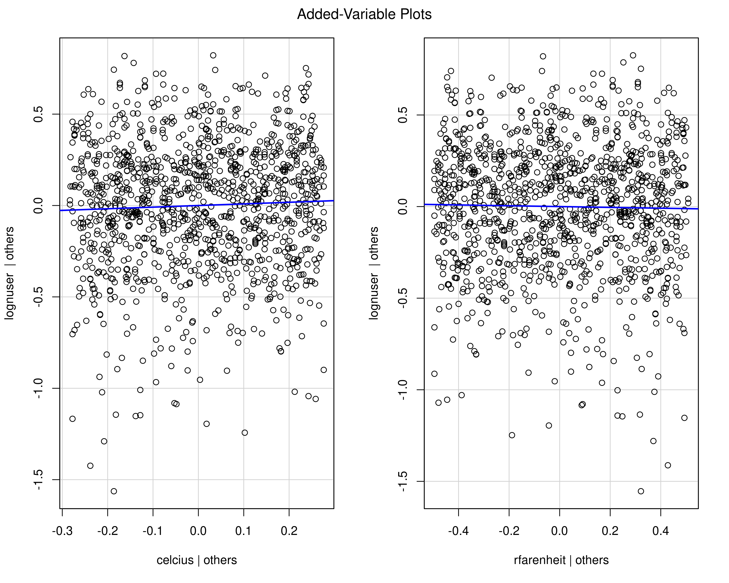
Added variable plots for Bixi multicollinearity data

Figure 1: Added variable plots for Bixi collinearity data. Both are collinear and show no relationship once either is included.
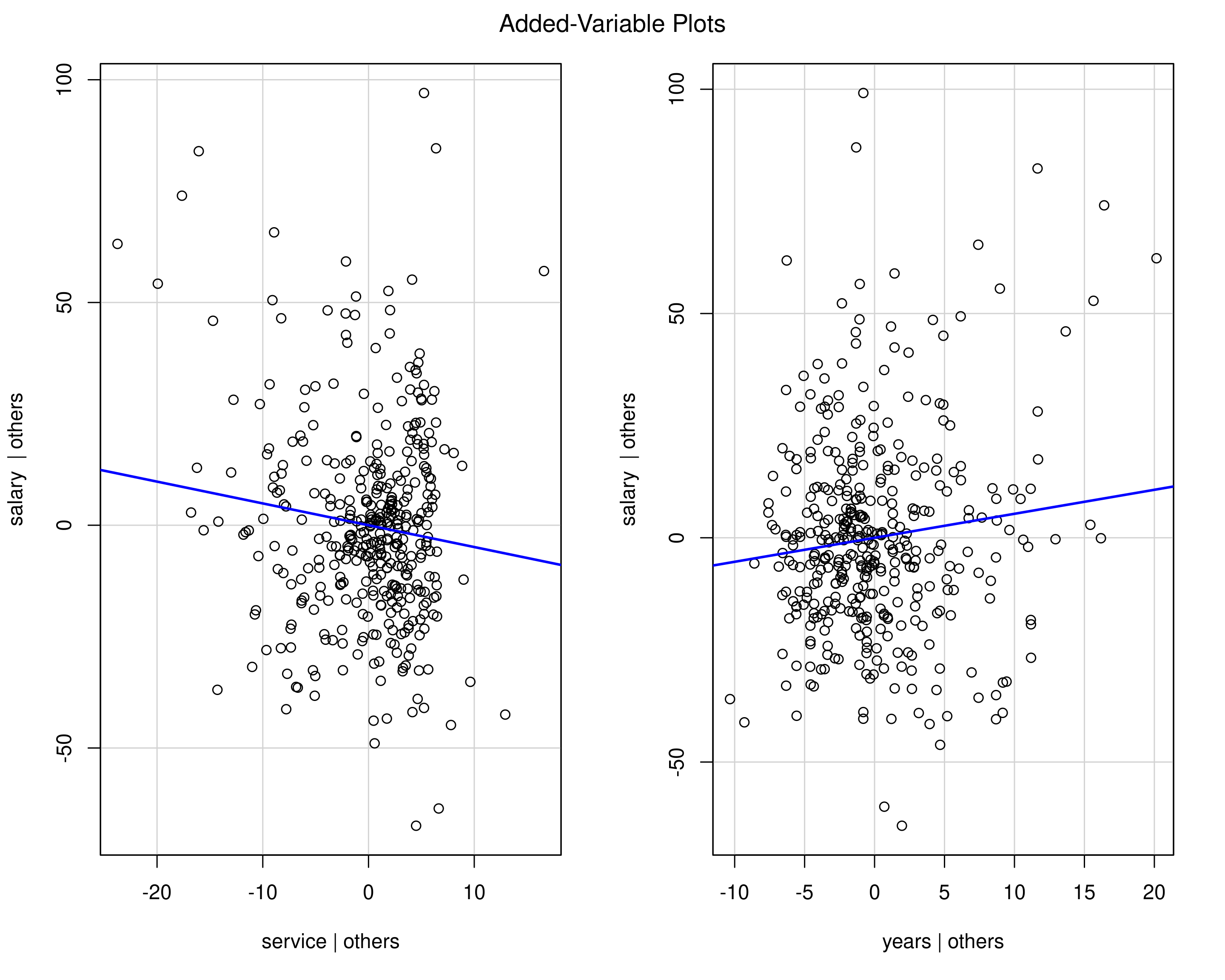
Example - added variable plots

Figure 2: Added variable plots for years of service and years since PhD. Both are collinear and show no relationship once either is included.
Confounding variable
A confounder is a variable \(C\) that is associated with both the response \(Y\) and an explanatory variable \(X\) of interest.
flowchart TD
    A("explanatory") --> B("response")
    C("confounder") --> A & B
    style A color:#FFFFFF, fill:#AA00FF, stroke:#AA00FF
    style B color:#FFFFFF, stroke:#00C853, fill:#00C853
    style C color:#FFFFFF, stroke:#2962FF, fill:#2962FF
The confounding variable \(C\) can bias the observed relationship between \(X\) and \(Y\), thus complicating the interpretations and conclusions of our analyses.
Example of confounder
The academic rank of professors is correlated with sex, because there are fewer women who are full professors and the latter are on average better paid. The variable rank is a confounder for the effect of sex.
| coef. | std. error | stat | p value | |
|---|---|---|---|---|
| intercept | 115.1 | 1.59 | 72.50 | < .001 |
| sex [woman] | -14.1 | 5.06 | -2.78 | .006 |
| coef. | std. error | stat | p value | |
|---|---|---|---|---|
| intercept | 81.59 | 2.96 | 27.56 | < .001 |
| sex [woman] | -4.94 | 4.03 | -1.23 | .220 |
| rank [associate] | 13.06 | 4.13 | 3.16 | .002 |
| rank [full] | 45.52 | 3.25 | 14.00 | < .001 |
Stratification and regression adjustment.
How to handle confounding variables? One way of discovering and accounting for a possible confounder is through stratification
- Compare salary separately for each rank (each rank consists of a stratum).
Or fit both variables in a regression model.
- We’ll be measuring the effect of
sex, adjusting for the other explanatory variables, which are possible confounders.
Experimental vs observational data
Confounders are really only an issue in the context of observational studies.
In experiments, randomization ensures balance across all confounders that could affect \(Y\).
In this case, we can thus make causal interpretations of the effect of \(X\) on \(Y\) without having to adjust for possible confounders.
