Estimators of the tail coefficient

Estimators proposed by Krupskii and Joe under second order expansion for the coefficient of tail dependence \(\eta\) and the joint tail orthant probability

Usage

kjtail(
  data,
  q,
  ptail = NULL,
  mqu,
  type = 1,
  ties.method = eval(formals(rank)$ties.method)
)

Arguments

data: a matrix of observations
q: vector of quantile levels
ptail: tail probability smaller than q. Default to NULL
mqu: marginal quantile levels for semiparametric estimation; data above this are modelled using a generalized Pareto distribution. If missing, empirical estimation is used throughout
type: integer indicating the estimator type
ties.method: method for ties

Value

a list with elements

p quantile level for estimation
eta estimated coefficient of tail dependence \(\eta\)
eta_sd estimated standard error of \(\eta\)
k1 parameter of the tail expansion
pat proportion of observations above the threshold
lambda tail dependence coefficient (sic)
tailprob tail probability, if ptail is provided

Note

EXPERIMENTAL. The numerical optimization of the likelihood surface is difficult, as the function is ill-behaved. Visual inspection of estimates is necessary to check for non-convergence.

Examples

d <- 2
rho <- 0.9
Sigma <- matrix(rho, d, d) + diag(1 - rho, d)
eta_true <- 1/sum(Sigma)
data <- mev::mvrnorm(
   n = 1e4,
   mu = rep(0, d),
  Sigma = Sigma)
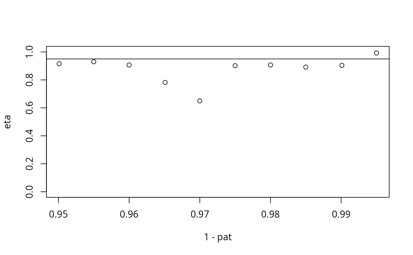
q <- seq(0.95, 0.995, by = 0.005)
taildep <- kjtail(data = data, q = q)
with(taildep,
 plot(x = 1-pat,
      y = eta,
      ylim = c(0,1),
      panel.first = {abline(h = (1+rho)/2)}))