1 Likelihood based inference for univariate extremes

1.1 Basic theory

Let \(\ell(\boldsymbol{y}; \boldsymbol{\theta})\) denotes the log-likelihood of an \(n\) sample with a \(p\)-dimensional parameter \(\boldsymbol{\theta}\). The score vector is \(U(\boldsymbol{\theta})=\partial \ell / \partial \boldsymbol{\theta}\), while the Fisher information is \(i(\boldsymbol{\theta})=\mathrm{E}\{U(\boldsymbol{\theta})U(\boldsymbol{\theta})^\top\}\). Under regularity conditions, we also have \(i(\boldsymbol{\theta}) = - \mathrm{E}(\partial^2 \ell / \partial \boldsymbol{\theta}\partial \boldsymbol{\theta}^\top)\). The observed information is the negative Hessian \(-\partial^2 \ell / \partial \boldsymbol{\theta}\partial \boldsymbol{\theta}^\top\), evaluated at the maximum likelihood estimator \(\hat{\boldsymbol{\theta}}\).

By definition, the maximum likelihood estimator solves the score equation, i.e. \(U(\hat{\boldsymbol{\theta}})=\boldsymbol{0}_p\). If the maximum likelihood estimator is not available in closed-form, its solution is found numerically and this property can be used to verify that the optimization routine has converged or for gradient-based maximization algorithms.

1.1.1 Likelihoods

There are four basic likelihoods for univariate extremes: the likelihood of the generalized extreme value (GEV) distribution for block maxima, the likelihood for the generalized Pareto distribution and that of the non-homogeneous Poisson process (NHPP) for exceedances above a threshold \(u\) and lastly the likelihood of the \(r\)-largest observations.

The generalized extreme value (GEV) distribution with location parameter \(\mu \in \mathbb{R}\), scale parameter \(\sigma \in \mathbb{R}_{+}\) and shape parameter \(\xi \in \mathbb{R}\) is \[\begin{align*} G(x) = \begin{cases} \exp\left\{-\left(1+\xi \frac{x-\mu}{\sigma}\right)^{-1/\xi}\right\}, & \xi \neq 0,\\ \exp \left\{ -\exp \left(-\frac{x-\mu}{\sigma}\right)\right\},& \xi = 0, \end{cases} \end{align*}\] defined on \(\{x \in \mathbb{R}: \xi(x-\mu)/\sigma > -1\}\) where \(x_{+} = \max\{0, x\}\). The case \(\xi=0\) is commonly known as the Gumbel distribution. We denote the distribution by \(\mathsf{GEV}(\mu, \sigma, \xi)\).

The generalized Pareto (GP) distribution with scale \(\sigma \in \mathbb{R}_{+}\) and shape \(\xi \in \mathbb{R}\) is \[\begin{align*} G(x) = \begin{cases} 1-\left(1+\xi \frac{x}{\sigma}\right)_{+}^{-1/\xi}, & \xi \neq 0,\\ 1- \exp \left(-\frac{x}{\sigma}\right),& \xi = 0. \end{cases} \end{align*}\] The range of the generalized Pareto distribution is \([0, -\sigma/\xi)\) if \(\xi < 0\) and is \(\mathbb{R}_{+}\) otherwise. We denote the distribution by \(\mathsf{GP}(\sigma, \xi)\).

Let \(Y_{(1)} \geq \cdots \geq Y_{(r)}\) denote the \(r\) largest observations from a sample. The likelihood of the limiting distribution of the point process for the \(r\)-largest observations is, for \(\mu,\xi\in\mathbb{R}, \sigma>0\), \[ \ell(\mu,\sigma,\xi; \boldsymbol{y}) \equiv -r\log(\sigma) - \left(1+\frac{1}{\xi}\right)\sum_{j=1}^r \log\left(1 + \xi\frac{y_{(j)}-\mu}{\sigma}\right)_{+} - \left(1 + \xi\frac{y_{(r)}-\mu}{\sigma}\right)^{-1/\xi}_+. \] This likelihood can be used to model the \(r\)-largest observations per block or threshold exceedances where the threshold is the \(r\)th order statistic

Consider a sample of \(N\) observations, of which \(n_u\) exceed \(u\) and which we denote by \(y_1, \ldots, y_{n_u}\). The likelihood associated to the limiting distribution of threshold exceedances is, for \(\mu, \xi \in \mathbb{R}, \sigma >0\), \[\begin{align} L(\mu, \sigma, \xi; \boldsymbol{y}) = \exp \left[ - c \left\{1+ \xi \left( \frac{u-\mu}{\sigma}\right)\right\}^{-1/\xi}_{+}\right] (c\sigma)^{-n_u}\prod_{i=1}^{n_u} \left\{1+\xi\left( \frac{y_i-\mu}{\sigma}\right)\right\}^{-1/\xi-1}_{+},\label{eq:ppp_lik} \end{align}\] where \((\cdot)_{+} = \max\{0, \cdot\}\). The quantity \(c\) is a tuning parameter whose role is described in 7.5 of Coles (2001). If we take \(c=N/m\), the parameters of the point process likelihood correspond to those of the generalized extreme value distribution fitted to blocks of size \(m\). The NHPP likelihood includes a contribution for the fraction of points that exceeds the threshold, whereas the generalized Pareto is a conditional distribution, whose third parameter is the normalizing constant \(\zeta_u=\Pr(Y>u)\). Since the latter has a Bernoulli and \(\zeta_u\) is orthogonal to the pair \((\sigma, \xi)\), it is often omitted from further analyses and estimated as the proportion of samples above the threshold.

1.1.2 Test statistics and the profile likelihood

The three main type of test statistics for likelihood-based inference are the Wald, score and likelihood ratio tests. The three main classes of statistics for testing a simple null hypothesis \(\mathrm{H}_0: \boldsymbol{\theta}=\boldsymbol{\theta}_0\) against the alternative \(\mathrm{H}_a: \boldsymbol{\theta} \neq \boldsymbol{\theta}_0\) are the likelihood ratio, the score and the Wald statistics, defined respectively as \[\begin{align*} w &= 2 \left\{ \ell(\hat{\boldsymbol{\theta}})-\ell(\boldsymbol{\theta}_0)\right\},\qquad \\w_{\mathsf{score}} &= U^\top(\boldsymbol{\theta}_0)i^{-1}(\boldsymbol{\theta}_0)U(\boldsymbol{\theta}_0),\qquad \\ w_{\mathsf{wald}} &= (\hat{\boldsymbol{\theta}}-\boldsymbol{\theta}_0)^\top i(\boldsymbol{\theta}_0)(\hat{\boldsymbol{\theta}}-\boldsymbol{\theta}_0), \end{align*}\] where \(\hat{\boldsymbol{\theta}}\) is the maximum likelihood estimate under the alternative and \(\boldsymbol{\theta}_0\) is the null value of the parameter vector. The statistics \(w, w_{\mathsf{score}}, w_{\mathsf{wald}}\) are all first order equivalent and asymptotically follow a \(\chi^2_p\) distribution, where \(q\) is the difference between \(p\) and the number of parameters under the null hypothesis. Under the conditions of the Neyman–Pearson theorem, the likelihood ratio test is most powerful test of the lot. The score statistic \(w_{\mathsf{score}}\) only requires calculation of the score and information under \(\mathrm{H}_0\), which can be useful in problems where calculations under the alternative are difficult to obtain. The Wald statistic \(w_{\mathsf{wald}}\) is not parametrization-invariant and typically has poor coverage properties.

Oftentimes, we are interested in a functional of the parameter vector \(\boldsymbol{\theta}\). The profile likelihood \(\ell_\mathrm{p}\), a function of \(\boldsymbol{\psi}\) alone, is obtained by maximizing the likelihood pointwise at each fixed value \(\boldsymbol{\psi}=\boldsymbol{\psi}_0\) over the nuisance vector \(\boldsymbol{\lambda}_{\psi_0}\), \[\begin{align*} \ell_\mathrm{p}(\boldsymbol{\psi})=\max_{\boldsymbol{\lambda}}\ell(\boldsymbol{\psi}, \boldsymbol{\lambda})=\ell(\boldsymbol{\psi}, \hat{\boldsymbol{\lambda}}_{\boldsymbol{\psi}}). \end{align*}\] We denote the restricted maximum likelihood estimator \(\hat{\boldsymbol{\theta}}_\psi= (\psi, \hat{\lambda}_{\psi})\).

We can define score and information in the usual fashion: for example, the observed profile information function is \[j_\mathrm{p}(\boldsymbol{\psi}) =-\frac{\partial \ell_\mathrm{p}(\boldsymbol{\psi})}{\partial \boldsymbol{\psi}\partial \boldsymbol{\psi}^\top} = \left\{j^{\boldsymbol{\psi\psi}}(\boldsymbol{\psi}, \hat{\boldsymbol{\lambda}}_{\boldsymbol{\psi}})\right\}^{-1}. \] The profile likelihood is not a genuine likelihood in the sense that it is not based on the density of a random variable.

We can turn tests and their asymptotic distribution into confidence intervals. For the hypothesis \(\psi = \psi_0\), a \((1-\alpha)\) confidence interval based on the profile likelihood ratio test is \(\{ \psi: 2\{\ell(\hat{\theta}) - \ell(\hat{\theta}_{\psi})\} \leq \chi^2_1(0.95)\}\).

Two typical questions in extreme values are: given the intensity of an extreme event, what is its recurrence period? and what is a typical worst-case scenario over a given period of time? For the latter, suppose for simplicity that the daily observations are blocked into years, so that inference is based on \(N\) points for the \(N\) years during which the data were recorded. The return level is a quantile of the underlying distribution corresponding to an event of probability \(p=1-1/T\) for an annual maximum, which is interpreted as ``the level exceeded by an annual maximum on average every \(T\) years’’. If observations are independent and identically distributed, then we can approximate the probability that a return level is exceeded \(l\) times over a \(T\) year period using a binomial distribution with probability of success \(1-1/T\) and \(T\) trials. For \(T\) large, the return level is exceeded \(l=0, 1, 2, 3, 4\) times within any \(T\)-years period with approximate probabilities 36.8%, 36.8%, 18.4%, 6.1% and 1.5%. The probability that the maximum observation over \(T\) years is exceeded with a given probability is readily obtained from the distribution of the \(T\)-year maximum, leading (Cox, Isham, and Northrop 2002, 3(b)) to advocate its use over return levels, among other quantities of interest such as the number of times a threshold \(u\) will be exceeded in \(T\) years or the average number of years before a threshold \(u\) is exceeded.

Quantiles, mean and return levels of \(T\)-maxima: consider the distribution \(H(x) = G^T(x)\) of the maximum of \(T\) independent and identically distributed generalized extreme value variates with parameters \((\mu, \sigma, \xi)\) and distribution function \(G\). By max-stability, the parameters of \(H(x)\) are \(\mu_T=\mu-\sigma(1-T^\xi)/\xi\) and \(\sigma_T=\sigma T^\xi\) when \(\xi \neq 0\). We denote the expectation of the \(T\)-observation maximum by \(\mathfrak{e}_T\), the \(p\) quantile of the \(T\)-observation maximum by \(\mathfrak{q}_p = H^{-1}(p)\) and the associated return level by \(z_{1/T} = G^{-1}(1-1/T)\). Then, any of these three quantities can be written as \[\begin{align*} \begin{cases} \mu-\frac{\sigma}{\xi}\left\{1-\kappa_{\xi}\right\}, & \xi <1, \xi \neq 0, \\ \mu+\sigma\kappa_0, & \xi =0, \end{cases} \end{align*}\] where \(\kappa_{\xi}=T^\xi\Gamma(1-\xi)\) for \(\mathfrak{e}_T\), \(\kappa_{\xi}=T^\xi\log(1/p)^{-\xi}\) for \(\mathfrak{q}_p\) and \(\kappa_{\xi}=\left\{-\log\left(1-{1}/{T}\right)\right\}^{-\xi}\) for \(z_{1/T}\). In the Gumbel case, we have \(\kappa_0=\log(T)+\gamma_{e}\) for \(\mathfrak{e}_T\), \(\kappa_0=\log(T)-\log\{-\log(p)\}\) for \(\mathfrak{q}_p\) and \(\kappa_0=-\log\{-\log(1-1/T)\}\) for \(z_{1/T}\).

1.2 Numerical example

This example illustrates some of the functions used in peaks-over-threshold analysis based on fitting a generalized Pareto distribution to threshold exceedances. We use the Venezuelian rainfall data, a time series of daily rainfall precipitations at Maiquetia airport in Venezuela, for the purpose of illustration.

library(mev)
data("maiquetia", package = "mev")
day <- seq.Date(from = as.Date("1961-01-01"), 
                to = as.Date("1999-12-31"), by = "day")
# Keep non-zero rainfall, exclude 1999 observations
nzrain <- maiquetia[substr(day, 3, 4) < 99 & maiquetia > 0]
gpdf <- fit.gpd(nzrain, threshold = 20)
print(gpdf)

## Method: Grimshaw 
## Log-likelihood: -832.629 
## 
## Threshold: 20 
## Number Above: 216 
## Proportion Above: 0.0604 
## 
## Estimates
##   scale    shape  
## 15.5800   0.1088  
## 
## Standard Errors
##   scale    shape  
## 1.60673  0.07785  
## 
## Optimization Information
##   Convergence: successful

We will ignore temporal dependence and stationarity, but these should be considered. The first step in our analysis is to choose a threshold. For the time being, we set the latter to 20 and consider threshold selection in the next section.

The default optimization routine for the generalized Pareto distribution is Grimshaw’s method, which profiles out the likelihood. The method has theoretical convergence guaranteesfor convergence. Because of non-regularity, the maximum likelihood estimator for \(\xi < -1\) does not solve the score equation and leads to infinite log-likelihood, hence the maximum returned lies on the boundary of the parameter space. The standard errors are based on the inverse observed information matrix and provided only if \(\xi>-1/2\). We can verify that our maximum likelihood estimate is indeed a maximum by checking if it solves the score equation if \(\hat{\xi}>-1\).

isTRUE(all.equal(
  gpd.score(gpdf$estimate, dat = gpdf$exceedances),
  c(0,0), tolerance = 1e-5))

## [1] TRUE

If the sample is small, maximum likelihood estimators are biased for the generalized Pareto distribution (the shape parameter is negatively biased, regardless of the true value for \(\xi\)). Bias correction methods includes the modified score of Firth, but the default method is the implicit correction (subtract), which solves the implicit equation \[\begin{align} \boldsymbol{\tilde{\theta}}=\hat{\boldsymbol{\theta}}-\boldsymbol{b}(\tilde{\boldsymbol{\theta}}). \label{eq:implbias} \end{align}\] The point estimate \(\boldsymbol{\tilde{\theta}}\) is obtained numerically as the root of this nonlinear system of equations. In the present case, the sample size is large and hence the first-order correction, derived through asymptotic arguments from the generalized Pareto distribution likelihood, is small. Note that the bias correction requires \(\xi > -1/3\), since it is based on third-order cumulants of the distribution.

gpdbcor <- gpd.bcor(dat = gpdf$exceedances, par = gpdf$estimate)
#print the differences between MLE and bias-corrected estimates
gpdf$estimate - gpdbcor

##      scale      shape 
##  0.1915284 -0.0118876

The package includes some default diagnostic plots (probability-probability plots and quantile-quantile plots), which include approximate confidence intervals based on order statistics. We can also get profile likelihood and profile-based confidence intervals for most quantities of interest (parameters of the generalized Pareto distribution, excepted shortfall, return levels, \(N\)-observation maxima mean and quantiles). The example below gives the estimated profile for the median of the centenial maximum distribution conditional on exceeding 15, along with 95% confidence intervals.

plot(gpdf, which = 2) #Q-Q plot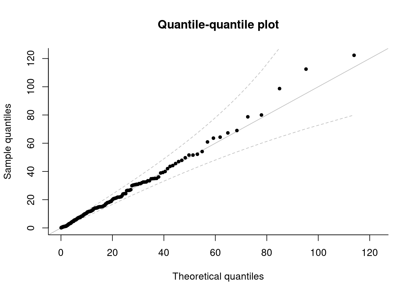

# Profile of median of maxima of 100 years
profile <- gpd.pll(param = "Nquant", dat = nzrain, threshold = 15, 
        N = length(nzrain)/(1998-1961)*100, q = 0.5)
# 95% confidence intervals
conf <- confint(profile, print = TRUE)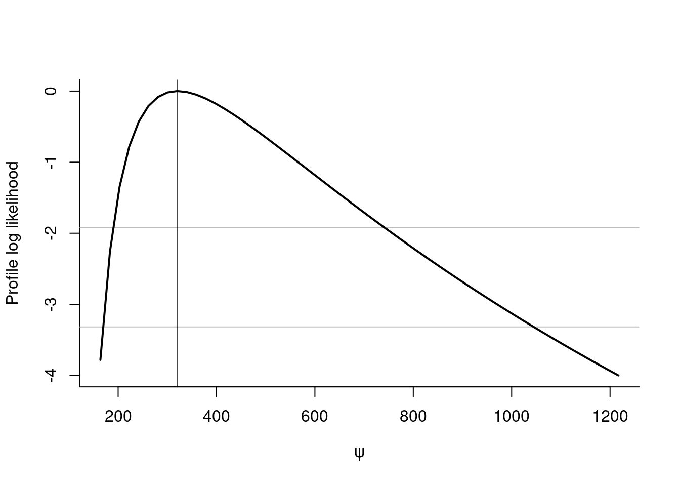

## Point estimate for the parameter of interest psi:
## Maximum likelihood          : 320.622 
## 
## Confidence intervals, levels : 0.025 0.975 
## Wald intervals               : 118.72 522.524 
## Profile likelihood           : 177.214 741.869

1.3 Your turn

Simulate 200 observations from the \(r\)-largest likelihood using rrlarg with shape parameter \(\xi=-0.2\) and \(r=5\).
Test the hypothesis \(\mathrm{H}_0: \xi = \xi_0\) using a score test and derive a 90% confidence interval for \(\xi\). You can obtain the maximum likelihood estimator by calling fit.rlarg and the score and information matrix are implemented under rlarg.score and rlarg.infomat. Recall that the score statistic \(w_{\mathsf{score}} \equiv U(\hat{\boldsymbol{\theta}}_{\xi_0})^\top i^{-1}(\hat{\boldsymbol{\theta}}_{\xi_0})U( \hat{\boldsymbol{\theta}}_{\xi_0}) \sim \chi^2_1.\)