3 Estimating the probability of rare events

Estimation of risk measures via Monte Carlo methods: simulate new replicates from the fitted model and compute number of points
For general risk regions where one or more component can be extreme, we proceed by fitting multiple conditional models
Entirely empirical approach

The whole point of estimating multivariate model is to estimate the probability of rare events. In general, we can estimate the probability of falling in a risk region $\mathcal{A} \subset\{Y_j > u_j\}$ via Monte Carlo simulations. In texmex, this is achieved with the predict method, which uses the model for simulation.

Under the hood, the function forms $n$ vectors of residuals \[ \widehat{\boldsymbol{z}}_{i|j} = y_{ij}^{-\widehat{\boldsymbol{\beta}}_{|j}}\left(\boldsymbol{y}_{i,-j} - \widehat{\boldsymbol{\alpha}}_{|j}y_{ij}\right), \quad (i=1, \ldots, n). \]

Then, choosing a threshold $v > u_j$, we can

Simulate $Y_j \sim \mathsf{Exp}(1) + v$.
Sample $\boldsymbol{z}_{|j}$ uniformly from the empirical distribution $\{\widehat{\boldsymbol{z}}_{i|j}\}_{i=1}^n$.
Set $\boldsymbol{Y}_{-j}= \widehat{\boldsymbol{\alpha}}Y_j + Y_j^{\widehat{\boldsymbol{\beta}}}\boldsymbol{z}_{|j}$.
Back-transform observations to original scale.

The predict method for objects of class mex and bootmex performs nsim=1000 replications by default above pqu=0.99. We may choose the dependence threshold over which to predict the other variables. Note that the bootstrap estimates contain in addition to the quantiles estimated standard error for the conditional mean. For the Fort Collins data, they appear to give much narrower quantile ranges.

The predict method includes an option smoothZdistribution to perform kernel smoothing for each marginal to remove artefacts. The levels of the conditional quantiles can be changed via the argument probs.

pred_boot <- predict(
    bootCondModFit, 
    pqu = 0.9,  
    trace = Inf)
# for the `bootmex` object, produces replications 
# for each bootstrap sample
pred_mex <- predict(condModFit, pqu = 0.9)
# `print` will output conditional mean
# `summary` gives conditional mean and quantiles
summary(pred_mex)
#> predict.mex(object = condModFit, pqu = 0.9)
#> 
#> Conditioned on precip being above its 90th percentile.
#> 
#> 
#> Conditional Mean and Quantiles:
#> 
#>      precip|precip>Q90 maxTemp|precip>Q90 minTemp|precip>Q90
#> mean              8.99              14.10               3.79
#> 5%                2.42              -2.25             -11.70
#> 50%               5.98              14.40               5.56
#> 95%              27.10              29.50              15.80
#> 
#> Conditional probability of threshold exceedance:
#> 
#>  P(precip>2.16|precip>Q90) P(maxTemp>30|precip>Q90)
#>                          1                    0.038
#>  P(minTemp>12.7778|precip>Q90)
#>                          0.158
summary(pred_boot)
#> predict.mex(object = bootCondModFit, pqu = 0.9, trace = Inf)
#> 
#> Results from 100 bootstrap runs.
#> 
#> Conditioned on precip being above its 90th percentile.
#> 
#> 
#> Conditional Mean and Quantiles:
#> 
#>      precip|precip>Q90 maxTemp|precip>Q90 minTemp|precip>Q90
#> mean             9.060             13.900              3.480
#> se               0.397              0.412              0.361
#> 5%               8.440             13.200              2.900
#> 50%              9.040             13.900              3.490
#> 95%              9.790             14.500              4.190
#> 
#> Conditional probability of threshold exceedance:
#> 
#>  P(precip>2.16|precip>Q90) P(maxTemp>30|precip>Q90)
#>                          1                   0.0335
#>  P(minTemp>12.7778|precip>Q90)
#>                          0.148

We can produce plots of predict.mex objects using ggplot. The resulting scatterplots are slightly confusing:

the orange full line gives the line $t_j(Y_j) = t_k(Y_k)$; since the data are plotted on the scale $(Y_j, Y_k)$ of the data, the line is curved.
the vertical dashed line represent the dependence threshold
grey points are original observations
blue diamonds are new simulated observations from the model for which the simulated conditioning variable $Y_j > Y_k$; orange circles are simulated points for which $Y_k > Y_j$.

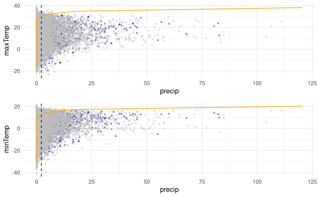
Simulations from the fitted conditional model above the 0.9 quantile (blue or orange) with original data (grey). The orange line indicates equal quantiles for the pair.

Figure 3.1: Simulations from the fitted conditional model above the 0.9 quantile (blue or orange) with original data (grey). The orange line indicates equal quantiles for the pair.

Thus, we can see that the simulation scheme produces coherent data in this case. The simulations are stored in pred_mex$data, a list which contains the original data (real), simulated observations on the data scale (simulated) and on the Laplace (transformed) scale.

We can access these data and compute empirical estimates of probabilities for various sets of interest.

Estimate the probability that the maximum daily temperature is below 30 degrees Celcius if the amount of rainfall is larger than 25 mm.

3.1 Self-consistency

So far, our model is only valid in the region $Y_j > u_j$, but more often than not we will be interested in more general events of the form $\{Y_j>u_j, Y_k>u_k\}$. Depending on the conditioning variable, we could express this in two ways: \[\begin{align*} \Pr(Y_k > u_k, Y_j > u_j) &= \Pr(Y_k > u_k \mid Y_j > u_j)\Pr(Y_j > u_j) \\& = \Pr(Y_j > u_j \mid Y_k > u_k)\Pr(Y_k > u_k) \end{align*}\] and if we choose a different conditioning variable, we will obtain different answers. This is one of the major drawback of the approach: it does not readily yield a genuine multivariate model and it is not self-consistent (meaning that the answer to the above question is the same regardless of the conditioning variable if $t_j(u_j) = t_k(u_k)$). For this to be the case, one would need to enforce additional constraints for $a_{j|k}=a_{k|j}$, etc.

3.2 Glue together conditional models

Heffernan and Tawn (2004) suggest splitting the risk region $\mathcal{A}$ into disjoint sets for exceedances, choosing the conditioning variable with the largest component on the Laplace scale. If we view the model as a mixture with adequate weights, this defines a valid multivariate distribution (cf. discussion of I. Papastathopoulos in Engelke and Hitz 2020), but the model fitting procedure does not factor this into account: it fits the model parameters $\boldsymbol{\alpha}_{|j}$ and $\boldsymbol{\beta}_{|j}$ with all data $\{\boldsymbol{Y}_i: Y_j>u_j\}$, not just that for which $\{\boldsymbol{Y}_i: Y_j>u_j, t_j(Y_j) > t_k(Y_k), k \neq j\}$.

The function mexAll fits all models conditional models together. One can then use mexMonteCarlo to generate points from each of these models, where in each case the $i$th bootstrap observation is replaced by a sample from the $j$th conditional extremes model, that is that for which $j$ is the largest standardized component occurs, i.e. $t_j(Y_{ij}) > t_k(Y_{ik})$ for $k \neq j$.

2 Multivariate model

References