2.1 Strength of extremal dependence

Before fitting the Heffernan-Tawn model, we can look at the strength of the extremal dependence between pairs.

We can first calculate the coefficient of tail dependence \(\chi\) and \(\overline{\chi}\) to investigate the strength of the extremal dependence.

The tail correlation coefficient \(\chi(u)\) is \[\chi(v)= \frac{\Pr\{F_1(Y_1) > v, F_2(Y_2)>v\}}{1-v}. \] and if \(\chi = \lim_{v \to 1} \chi(v) >0\), we say that \((Y_1, Y_2)\) are asymptotically dependent. Since \(\chi=0\) for all asymptotically independent process, this is not useful measure.

The tail dependence coefficient (Coles, Heffernan, and Tawn 1999) \(\bar{\chi}\) is estimated using \[\begin{align*} \bar{\chi}(v) = \frac{2\log(1-v)}{\log[\Pr\{F_1(Y_1) > v, F_2(Y_2) > v\}}-1 \end{align*}\] for \(v \in (0,1)\), so \(\overline{\chi} \in [-1,1]\) and asymptotically dependent processes have \(\lim_{v \to 1} \overline{\chi}(v)=1\). The statistic \(\chi\) is only useful when the data are asymptotically dependent, so we normally look first at \(\overline{\chi}\) and if the Wald confidence intervals include 1, look at the strength of the dependence using the plot of \(\chi\). The texmex package will gray out the latter if asymptotic dependence is ruled out.

# Create plot with matrix or data frame
#  with 2 columns only
chiplot_13 <- 
  chi(FortCollins[,c("maxTemp","precip")])
chiplot_23 <- 
  chi(FortCollins[,c("minTemp","precip")])

# Truncated the plots to focus on the upper right tail
# because most of the rainfall records are zero
ggplot(chiplot_13, xlim = c(0.9,1))
ggplot(chiplot_23, xlim = c(0.9,1))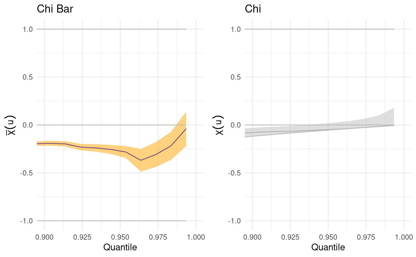

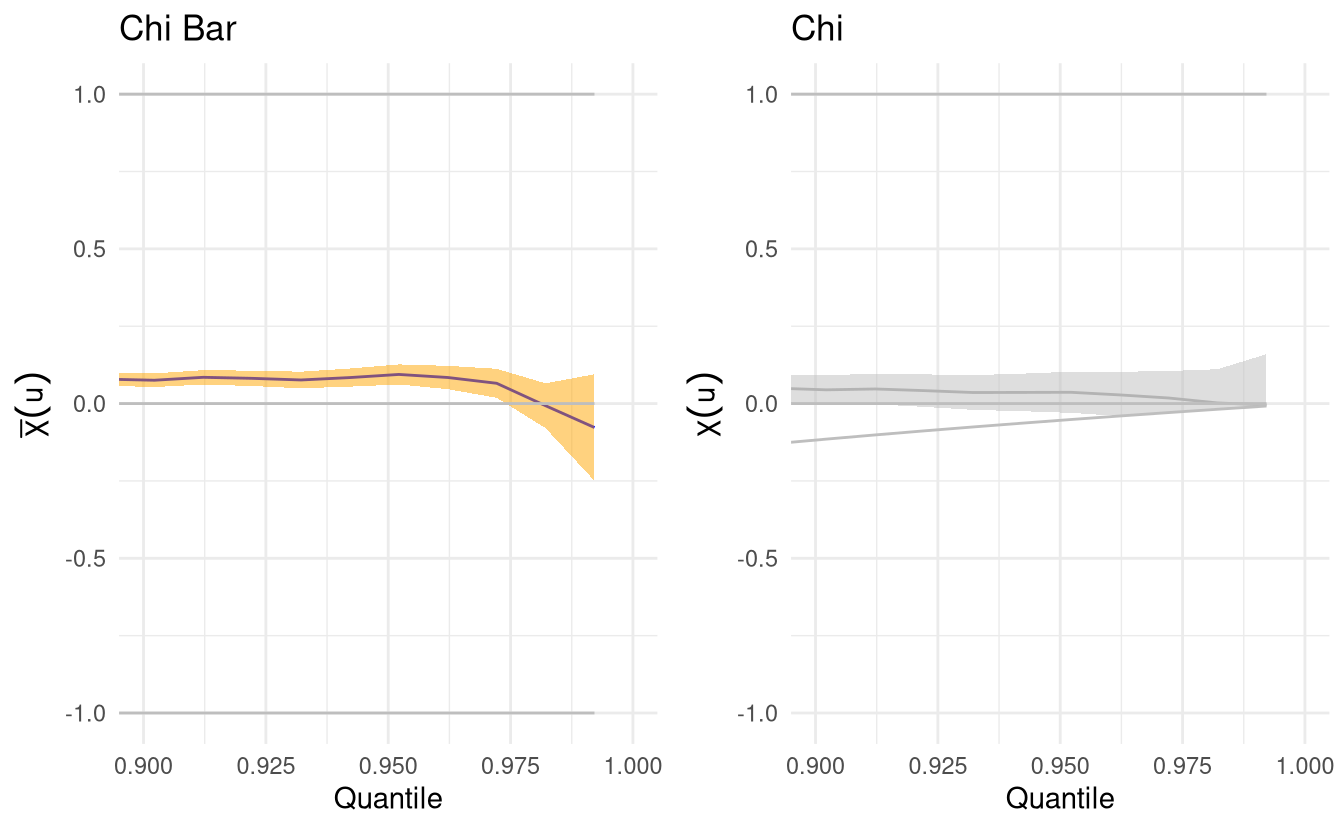
Figure 2.1: Tail dependence plots for maximum daily temperature (top panel) and minimum daily temperature (bottom panel), conditional on extreme rainfall. The right-hand panel is greyed out if asymptotic dependence has been ruled out.

If the conditional extremes model holds, then \(t_k(Y_{k}) \mid t_j(Y_{j}) > t_j(u_j)\) can be approximated by \(\widetilde{Y}^*_{k|j} \approx \alpha_{k|j}t_j(Y_j)+t_j(Y_j)^{\beta_{k|j}}Z_{k|j}\). We thus obtain a formula for \(\chi(v)\) above the dependence threshold \(u^{\star}=t_j(u)\), where for any \(v^{\star}=-\log\{2\cdot(1-v)\}\) \((v > 0.5)\) such that \(v^{\star} > u^{\star}\), we have \[\begin{align} \chi(v) = \tfrac{\Pr\{t_j(Y_j) > u^{\star}\}\Pr\{\widetilde{Y}^{\star}_{k|j} > v^{\star}, t_j(Y_j) > v^{\star}, t_j(Y_j) > v^{\star} \mid t_j(Y_j) > u^{\star}\}}{\Pr\{t_j(Y_j) > v^{\star}\}} \label{HTchi} \end{align}\] We can estimate empirically the coefficient of tail dependence by resampling values of \(Z_{k|j}\). The values are simulation-based, so we can use the average over many replications. This does not factor into account the parameter uncertainty, which would require using the bootstrap.

The texmex package also includes a multivariate conditional estimator of Spearman’s \(\rho\) (linear correlation on the scale of \(F_1(Y_1), \ldots, F_D(Y_D)\)). The function MCS computes the estimator, whereas bootMCS can be used to get a measure of uncertainty by running a nonparametric bootstrap and computing 95% pointwise confidence intervals.

2.2 Fitting the multivariate model

The main function for fitting the conditional extreme value model in texmex is mex which gives the two stage procedure and calls internally.

• First, migpd fits a generalized Pareto distribution to each margin. Users must provide
  • mth or mqu: either the thresholds \(u_1, \ldots, u_D\) (argument mth) or else a vector of probability levels \(F_1(u_1), \ldots, F_D(u_D)\) (argument mqu)
  • User can compute the maximum a posteriori (instead of the maximum likelihood estimates) for parameters, with \(\log(\tau) \sim \mathsf{No}(0,100)\) independent of \(\xi \sim \mathsf{No}(0,0.25)\) as default prior specifications if penality='gaussian' (the default).
• These standardized data are fed to mexDependence. The latter has multiple arguments:
  • which: the column index for the conditioning variable
  • dqu: the probability level of the marginal quantile at which to specify \(t(\boldsymbol{Y}) \mid t_j(Y_j) > t_j(u_j)\); note that this threshold need not be the same as the marginal threshold for the generalized Pareto.
  • margins the choice of distribution for the standardisation (default is ‘laplace’)
  • marTransform: how to model \(F_k\) to transforms every component of \(\boldsymbol{Y}\) to standard Laplace margins. The default, marTransform="mixture" use the semiparametric transformation (the data are modelled with the empirical distribution below the threshold and with a generalized Pareto above \(u\)). The alternative is to use the empirical distribution (marTransform = "empirical").
  • constrain whether to impose constraints to improve self-consistency for estimates of \(\boldsymbol{a}_{|j}\) and \(\boldsymbol{b}_{|j}\); defaut is TRUE;
  • PlotLikDo logical; whether to produce a bivariate profile likelihood defined on a curved subset of \([-1,1] \times[-\infty, 1]\) if constrain=TRUE.

In general, unless you want to obtain the profile likelihood plot, you could directly use mex which combines these two steps.

Once we have determined marginal and functional thresholds and the choice of conditioning variable, we can perform all steps at once using mex.

marg <- 
  FortCollins %>% 
  select(!date) %>% 
  migpd(
    mqu = rep(0.9, 3), 
    penalty = 'none'
    )
condModFit <- 
  mexDependence(
    x = marg,
    which = "precip", 
    dqu = 0.9, 
    PlotLikDo = FALSE,
    PlotLikRange = list(a = c(-1, 1),
                        b = c(-3, 1))
    )
print(condModFit)
#> mexDependence(x = marg, which = "precip", dqu = 0.9, PlotLikDo = FALSE, 
#>     PlotLikRange = list(a = c(-1, 1), b = c(-3, 1)))
#> 
#> 
#> Marginal models:
#> 
#> Dependence model:
#> 
#> Conditioning on precip variable.
#> Thresholding quantiles for transformed data: dqu = 0.9
#> Using laplace margins for dependence estimation.
#> Constrained estimation of dependence parameters using v = 10 .
#> Log-likelihood = -5996 -6160 
#> 
#> Dependence structure parameter estimates:
#>   maxTemp minTemp
#> a  0.0201   0.160
#> b -0.6488  -0.401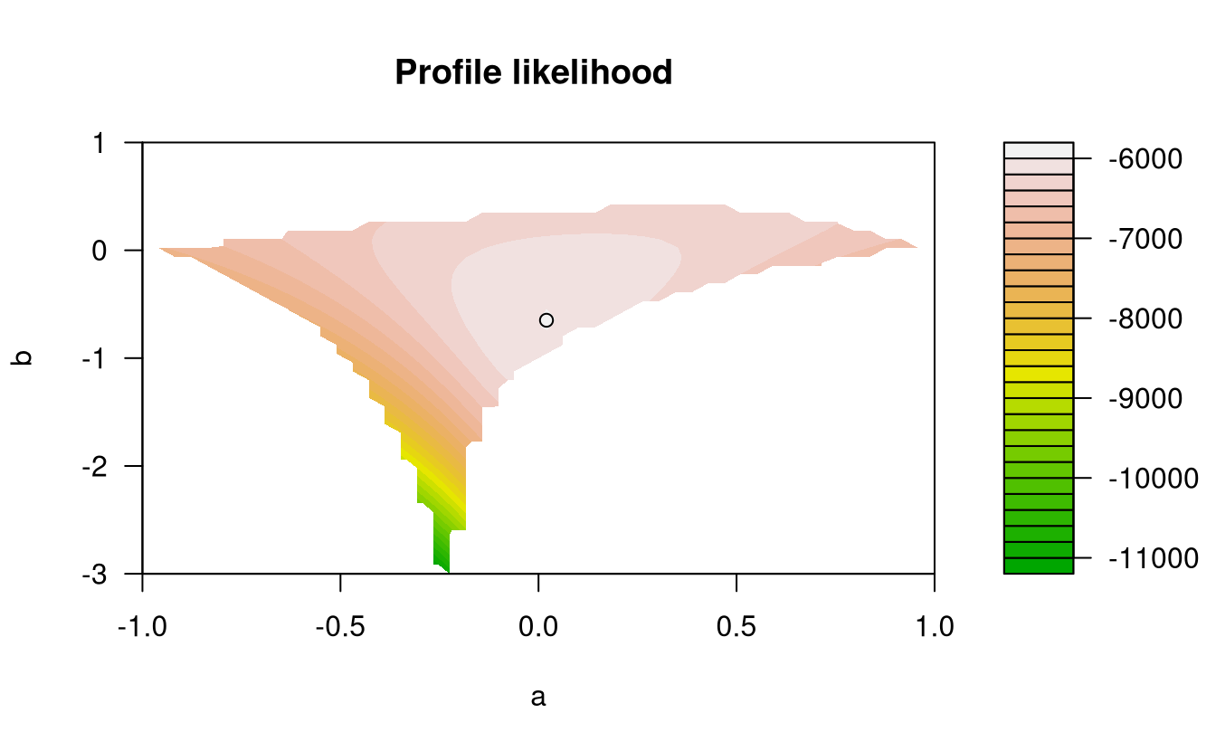

We can show that the components \(Y_j\) and \(Y_k\) are:

• asymptotically dependent only if \(\alpha_{k|j}=1\), \(\beta_{k|j}=0\)
• asymptotically independent if \(-1<\alpha_{k|j}<1\)
  • positive extremal dependence if \(\alpha_{k|j}>0\)
  • negative extremal dependence if \(\alpha_{k|j}<0\)
  • near independence if \(\alpha_{k|j}=\beta_{k|j}=0\). Negative values of \(\beta\) (\(b\) in the plots) imply that all if the conditional quantiles of \(Y_k\) converge to the same value as \(Y_j\). This is often implausible.

2.3 Functionalities of mex and diagnostic plots

The output of mex or mexDependence is an object of class mex, for which many S3 methods are available (including print and summary). By default the plot (or ggplot) method produce diagnostic plots of

• standardized residuals \(\widehat{Z}_k(Y_j)\) against \(\widehat{F}_j(Y_j)\) with lowess curve
• absolute value of standardized residuals against \(\widehat{F}_j(Y_j)\)
• plot of \(Y_k\) against \(Y_j\) with fitted quantiles

If there is a trend, this contradicts somewhat the assumption that the residuals \(Z\) are independent of the value of \(Y_j\), and perhaps suggest that the threshold used for the dependence is too low.

ggplot(condModFit)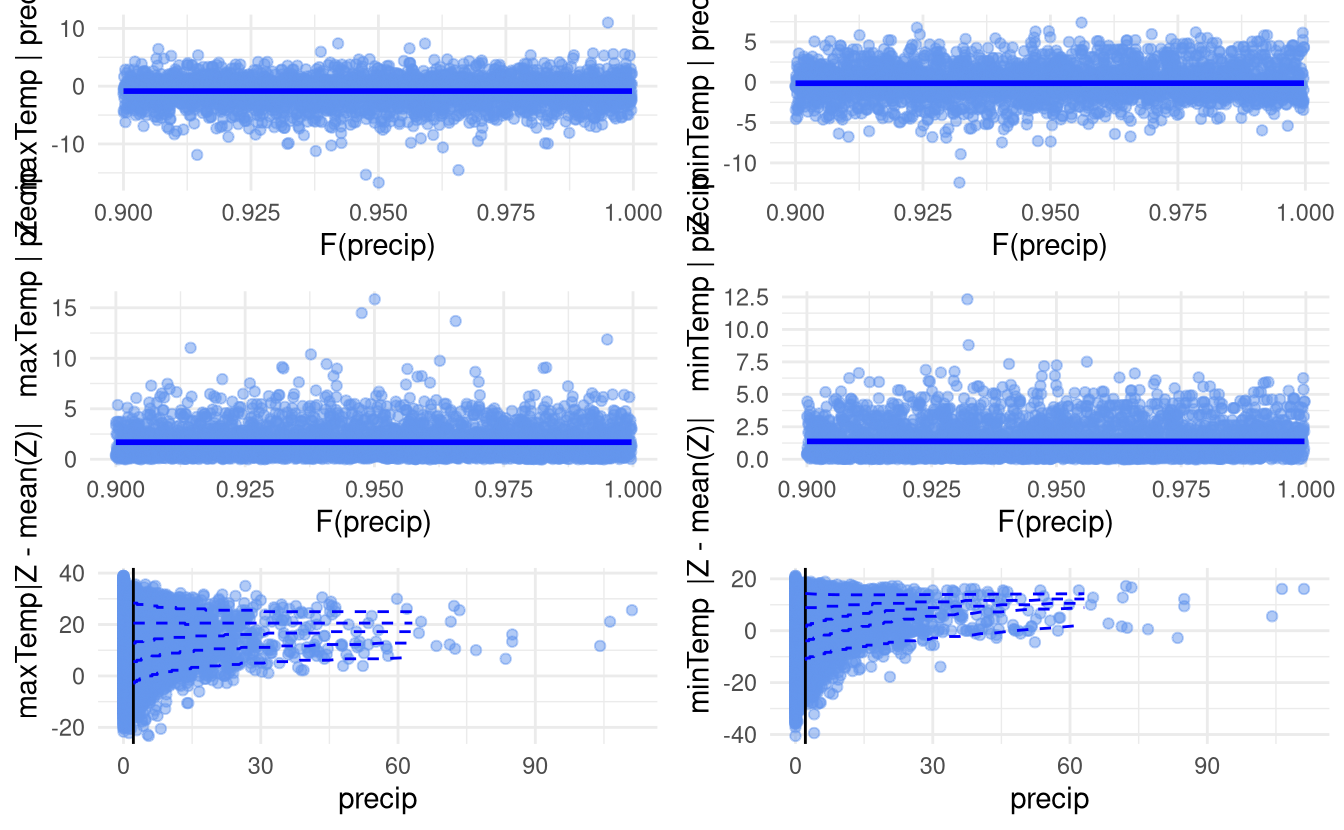

Figure 2.2: Regression diagnostic plots for the fitted conditional extremes model.

2.4 Uncertainty quantification

The drawback of the “bricolage” approach for model fitting is that we do not have readily available uncertainty quantification. Heffernan and Tawn address this by devising a semiparametric bootstrap scheme. It consists of the following steps:

• obtain nonparametric bootstrap sample (with replacement) from \(\{\boldsymbol{Y}_i, \ldots, \boldsymbol{Y}_n\}\)
• obtain \(D\) samples of size \(n\) from the standard Laplace margins \(\boldsymbol{Z}^{(b)}\).
• reorder Laplace observations of each margin so that their rank match that of the nonparametric bootstrap.
• transform observations to the data scale using \(\widehat{F}_j^{-1}(\cdot)\) \((j=1, \ldots, D)\)

Thus, we have a new dataset from which to estimate the dependence. Rince and repeat every step including

• empirical distribution estimation
• generalized Pareto above threshold
• multivariate model with coefficients

The bootmex package takes the output of mex or mexDependence and produces R replicates.

bootCondModFit <- bootmex(condModFit)

So far, we have not assessed the choice of threshold for the procedure. We can produce a threshold stability plot by fitting the model over a range of values of dqu and look at the resulting estimates. This, coupled with some bootstrap replicates, is useful to make sure the optimization algorithm did converge and that the threshold is high enough for the approximation to hold.

threshold_stab_multi <-
  mexRangeFit(
    x = marg, 
    quantiles = seq(0.90, 0.98, by = 0.02),
    which = "precip", #margin to condition on
    R = 10L, # number of bootstrap samples
    trace = Inf
  )
ggplot(threshold_stab_multi)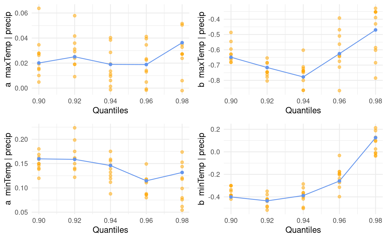

Figure 2.3: Dependence threshold stability plots with 10 bootstrap replicates for the conditional extreme value model fitted above the 0.9 quantile of cumulated daily precipitation.

We can use the resulting object to produce scatterplots of pairs of parameter estimates for each margin and get bootstrap confidence intervals or standard errors for the parameters.

# ggplot method seems broken...
par(mfrow = c(1,2), bty = "l")
plot(bootCondModFit, plot = "dependence")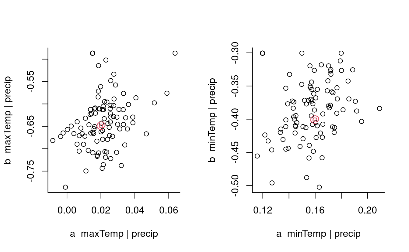

Figure 2.4: Scatterplot of bootstrap parameter estimates for the coefficients of the conditional extreme value model for maximum daily temperature (left) and minimum daily temperature (right) conditional on cumulated daily precipitation. The maximum likelihood estimate for the original data is indicated with the at-sign (red).