1 Marginal distribution and generalized Pareto tails
- Fit marginal models with generalized Pareto tails and empirical distribution for the body of the data.
- Pick suitable thresholds for generalized Pareto distribution using diagnostic plots
The conditional extremes model attempts to describe the general behaviour of a \(D\) random vector \(\boldsymbol{Y}\) when component \(Y_j\) exceeds a high threshold \(u_j\). This parallels other multivariate peaks-over-threshold models, including the multivariate generalized Pareto distributions arise as the limiting distribution given that \(\max_{j=1}^D Y_j > u_j\) under an hypothesis of regular variation and the \(R\)-Pareto processes when \(R(\boldsymbol{Y})>u\) for a one-homogeneous functional \(R\).
Univariate extreme value theory suggests that \(Y_j \mid Y_j > u_j\) can be approximated by a generalized Pareto distribution with scale \(\tau\) and shape \(\xi\) above \(u_j\) and we can proceed likewise for other components of \(\boldsymbol{Y}\). However, it is worth keeping in mind that the other components of \(\boldsymbol{Y}\) need not be simultaneously large when \(Y_j>u_j\). Rather than specify a parametric model for \(Y_k\) \((k \neq j)\), we can use the empirical distribution, \[\begin{align*} F^{(k)}_n(y) = n^{-1}\sum_{i=1}^n \mathrm{I}(y \leq y_{ik}) \end{align*}\] or a semiparametric alternative \[\begin{align*} \widehat{F}_k(y) = \begin{cases} F{(k)}_n(y) & y \leq u_k; \\ 1-\{1-F^{(k)}_n(u_k)\}\left(1+\xi_k\frac{y-u_k}{\tau_k}\right)^{-1/\xi_k}_{+} & y > u_k. \end{cases} \end{align*}\] to model the marginal distribution. This leaves the matter of the dependence structure.
1.1 Threshold selection
To determine which threshold to select for marginal exceedances, we can produce threshold stability plots: these consist of shape estimates (with pointwise 95% confidence intervals, even if these are presented as bands) over a range of thresholds \(u_1 < \cdots < u_m\). Assuming the generalized Pareto approximation to be adequate at \(u_l\), the estimates should stabilize for thresholds \(u_{l+1}, \ldots, u_m\) (Davison and Smith 1990).
thstab <-
  with(FortCollins,
     texmex::gpdRangeFit(
       data = precip,
       umin = 20,
       umax = 50,
       nint = 10L,
       penalty = "none")
     # alternative is 'gaussian', yielding MAP
)
# there are two methods for graphics:
# plots (base R) or ggplot (ggplot2)
patchwork::wrap_plots(ggplot(thstab))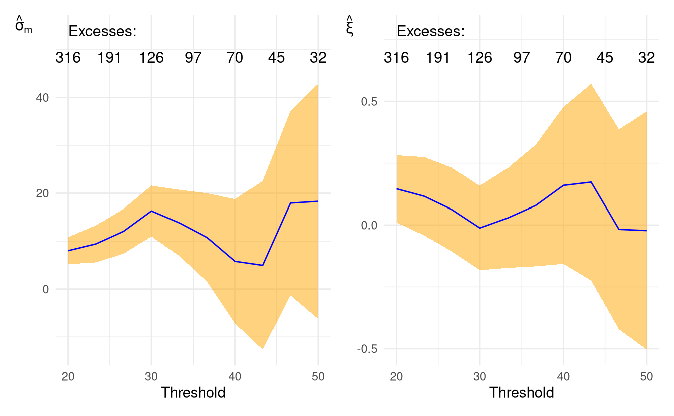
Figure 1.1: Threshold stability plots for adjusted scale (left) and shape parameter (right) for the Fort Collins daily cumulated precipitation.
While the shape estimates decrease steadily as we increase the threshold, it seems here that 25mm is a reasonable marginal threshold for rainfall.
The function mrl produces mean residual life plots ggplot(texmex::mrl(data = precip)), but the literature on graphics suggests the human eye has a much easier time detecting lack of trend than linearity.
- Repeat the exercise, this time with daily minimum and maximum temperature.
- For the chosen threshold, fit a generalized Pareto using the function
evmwith thresholdth. You can explore the different methods (maximum likelihood, penalized maximum likelihood, Bayesian estimation with Markov chain Monte Carlo using independent elliptical proposals) - Produce a quantile-quantile plot to check the goodness of fit (via
plotorggplotfor the object returned byevm).
1.2 Standardization of the margins
The Heffernan-Tawn model describes extremes for standardized data, but there is a direct correspondence between extremes \(\{\boldsymbol{Y}: Y_j > u_j\}\) and \(\{\boldsymbol{Y}: t_j(Y_j) > t_j(u_j)\}\) for a monotone transformation \(t_j\). The standardization in Heffernan and Tawn (2004) is to the Gumbel scale, but subsequent work (Keef, Papastathopoulos, and Tawn 2013) suggests a better choice is standard Laplace, i.e., a distribution with double exponential tails that can capture negative and positive dependence.
The standard Laplace distribution has density \(f(x) = \exp(-|x|)/2\) on \(\mathbb{R}\) and distribution function \[\begin{align*} F(x) = \begin{cases} \frac{1}{2}\exp(x) & x < 0, \\ 1-\frac{1}{2}\exp(-x) & x \geq 0. \end{cases} \end{align*}\] Thus, if \(Y_1, \ldots, Y_D\) is a random vector with marginal distribution functions \(F_1, \ldots, F_D\), we can make the margins standard Laplace by applying the quantile transformation \[\begin{align*} t_k(Y_k) = \begin{cases} \log\{2{F}_k(Y_k)\} & {F}_k(Y_k) < 1/2, \\ -\log[2\{1-{F}_k(Y_k)\}] & {F}_k(Y_k) \geq 1/2, \end{cases} \qquad k=1, \ldots, D. \end{align*}\] In practice, we replace the unknown \(k\)th marginal distribution function \(F_k\) by the semiparametric estimator \(\widehat{F}_k\).