Statistical inference
The renfe data contains information about 10 000 train ticket sales from Renfe, the Spanish national train company. The data include:
price: price of the ticket (in euros);dest: binary variable indicating the journey, either Barcelona to Madrid (0) or Madrid to Barcelona (1);fare: categorical variable indicating the ticket fare, one ofAdultoIda,PromoorFlexible;class: ticket class, eitherPreferente,Turista,TuristaPlusorTuristaSolo;type: categorical variable indicating the type of train, either Alta Velocidad Española (AVE), Alta Velocidad Española jointly with TGV (parternship between SNCF and Renfe for trains to/from Toulouse and beyond)AVE-TGVor regional trainREXPRESS; only trains labelledAVEorAVE-TGVare high-speed trains.duration: length of train journey (in minutes);wdayinteger denoting the week day, ranging from Sunday (1) to Saturday (7).
Exercise 1.1
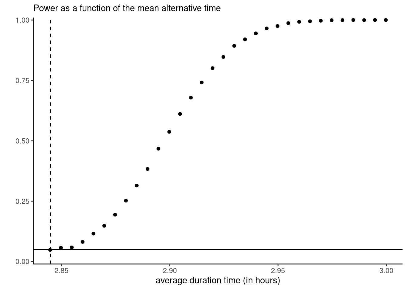
We consider travel time for high-speed (AVE and AVE-TGV) trains. The true “population” mean travel time between cities is known to be \(\mu=2.845\) hours (the instructor has access to the full dataset of more than 2.3 millions records, so these are known quantities, unlike in most practical settings).
A simulation study is performed to assess the behaviour of univariate tests under repeated sampling. The following algorithm was repeated 10K times for different values of \(\mu_0\):
- Select a random subsample of size \(n=100\).
- Compute the one-sample \(t\)-test statistic for \(\mathscr{H}_0: \mu=\mu_0\) (versus \(\mathscr{H}_0: \mu \neq \mu_0\)) .
- Return the \(p\)-value
Figure 1 shows the percentage of the 10K \(p\)-values that are less than 0.05, i.e. the percentage of rejection (at the \(5\)% level) of \(\mathscr{H}_0:\mu=\mu_0\) against the two-sided alternative at \(\mu_0 \in \{2.83, \nu, 2.835, 2.84, \ldots, 2.995, 3\`\). Use the resulting curve to answer the following questions:
- Explain why the value for the one-sample \(t\)-test around \(\mu=2.845\) should be approximately 0.05.
- Explain why the values on the curve increase towards the right of the plot.
- Suppose we repeated the simulation study, but this time with subsamples of size \(n=1000\). How would the points compare for the one-sample \(t\)-test: should they be higher, equal, or lower than their current values?
- Is the assumption of the one-sample \(t\)-test valid in this example? Produce a quantile-quantile plot using the code below and hence comment on the robustness of the \(t\)-test to departures from the normality assumption.
Exercise 1.2
Suppose we now want to compare the mean fare for high-speed train tickets for the two destinations, i.e., Madrid to Barcelona versus Barcelona to Madrid. We run a simulation study where we perform a two-sided Welch test for this hypothesis repeatedly with random subsamples of size \(n=1000\). The data renfe_simu contains the mean difference (meandif), the test statistic (Wstat), the \(p\)-value (pval) and the confidence interval (cilb and ciub) for these 1000 repetitions. Based on the entire database, the true mean difference is known to be \(-0.28\)€. Use the simulated data to answer the following questions and briefly comment on each item
- What is the empirical coverage of the 95% confidence intervals (i.e., the percentage of intervals covering the true mean difference value)?
- Plot an histogram of the mean differences and superimpose the true mean difference in the population.
- Compute the power of the test (percentage of rejection of the null hypothesis).
Exercise 1.3
Using the renfe data, test whether the average ticket price of AVE-TGV trains is different from that of Regio Express trains (REXPRESS). Make sure to
- State your null and alternative hypothesis.
- Carefully justify your choice of test statistic.
- Report the estimated mean difference and a 90% confidence interval for that difference.
- Conclude within the setting of the problem.