The level of the test is 5%, so we should reject 5% of the time under the null.
The curve is the power curve, i.e., the percentage of rejection of the null hypothesis for one-sample \(t\)-test. The further away from the true value \(\mu\), the higher the ability to detect departures from \(\mathscr{H}_0\). Because we set \(\alpha=0.05\), the curve should be around 0.05 near \(\mu\) and increase towards 1 as we move away from the true population mean.
Power increases if the sample size \(n\) increases, so we expect to see the curve be higher everywhere, but at \(\mu\) where it should be close to \(0.05\) if the test is calibrated.
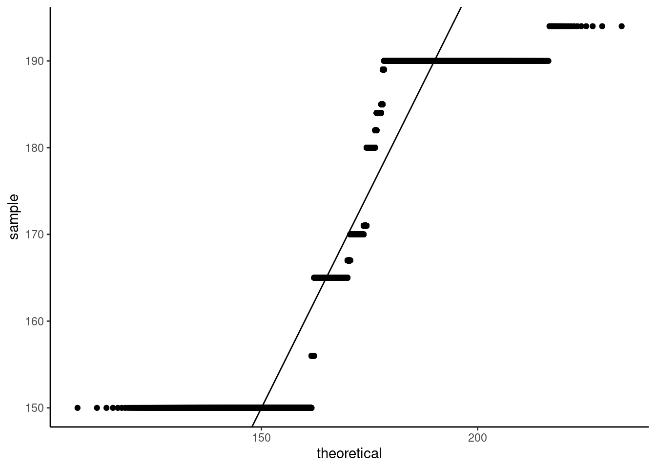
The data are clearly not symmetric and heavily discretized, yet the power curve of the one-sample \(t\)-test is steadily increasing and the nominal level matches the type I error. This illustrates the robustness of the test to departures from normality.
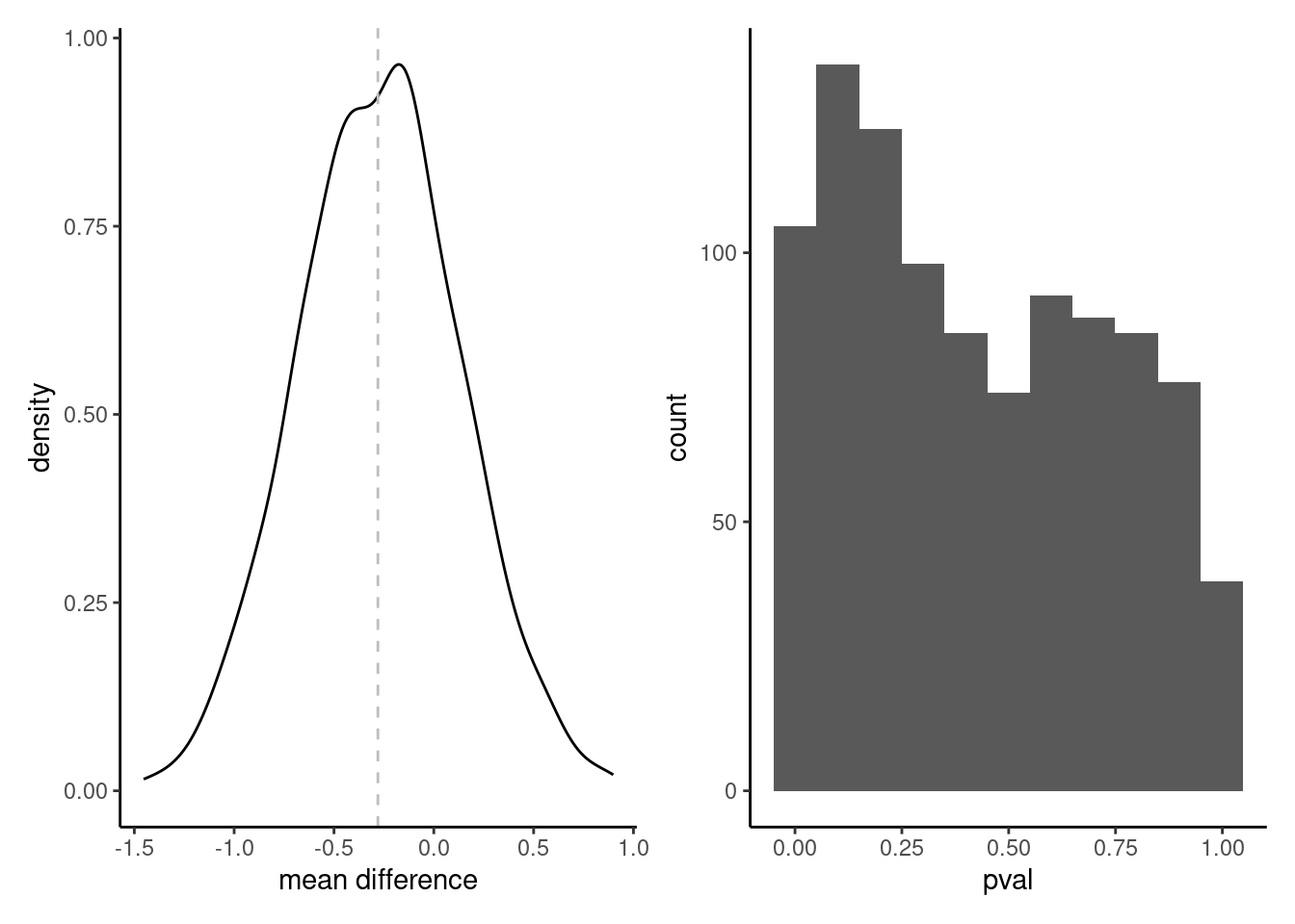
The histogram for the mean difference in Figure 1 looks symmetric and light-tailed, and centered around 0.28, whereas the \(p\)-values are scattered in the unit interval, with some values closer to zero.
Figure 1: Left: density plot of the mean difference price for high-speed train tickets from Madrid to Barcelona versus Barcelona to Madrid, along with average (gray vertical line). Right: histogram of p-values.
The power is \(0.105\). Under the alternative regime (since \(\Delta=0.28\)€), we only reject 10.5% of the time. While this number is low, it is due to the small size of the true mean difference, which is hard to detect unless the sample size is enormous. The estimated mean difference for the sample is \(0.274\)€.
Code
t.test(price ~ dest, data = renfe_sub)
    Welch Two Sample t-test

data:  price by dest
t = -1.9433, df = 9170.2, p-value = 0.05201
alternative hypothesis: true difference in means between group Barcelona-Madrid and group Madrid-Barcelona is not equal to 0
95 percent confidence interval:
 -1.652691253  0.007157275
sample estimates:
mean in group Barcelona-Madrid mean in group Madrid-Barcelona
                      87.40053                       88.22329
Code
mean(renfe_simu$pval <0.05)
[1] 0.105
Solution to Exercise 1.3
Careful here, as the price of the REXPRESS tickets is fixed at 43.25€. The only random sample is for the other class of train!
Code
with(renfe,t.test(x = price,mu =43.25,conf.level =0.9,subset = type =="AVE-TGV"))
    One Sample t-test

data:  price
t = 197.9, df = 9999, p-value < 2.2e-16
alternative hypothesis: true mean is not equal to 43.25
90 percent confidence interval:
 85.73892 86.45119
sample estimates:
mean of x
 86.09505
The null hypothesis is \(\mathscr{H}_0: \mu_{\text{AVE-TGV}}=43.25\)€ against the alternative \(\mathscr{H}_1: \mu_{\text{AVE-TGV}}\neq 43.25\)€, where \(\mu_{\text{AVE-TGV}}\) is the average AVE-TGV ticket price.
Since this is a one-sample location problem, we use a one-sample \(t\)-test.
The estimated mean difference is \(45.63\)€\(= 88.88\)€\(-43.25\)€, with 90% confidence interval for the mean difference of \([44.14, 47.12]\).
The \(t\)-statistic is 50.519 with 428 degrees of freedom, and the \(p\)-value is negligible.
We strongly reject the null hypothesis that high-speed trains are the same price as RegioExpress ones.