1.7 Solutions to Exercises

1.7.1 Solutions 1: Beaver temperature

Load the beav2 data from the library MASS.
Examine the data frame using summary, head, tail. Query the help with ?beav2 for a description of the dataset
Transform the temperature data into a time series object and plot the latter.
Fit a linear model using lm and the variable activ as factor, viz. lin_mod <- lm(temp~as.factor(activ), data=beav2). Overlay the means on your plot with lines(fitted(lin_mod)) replacing lin_mod with your lm result.
Inspect the residuals (resid(lin_mod)) and determine whether there is any evidence of trend or seasonality.
Look at a quantile-quantile (Q-Q) plot to assess normality. You can use the command qqnorm if you don’t want to transform manually the residuals with qqline or use plot(lin_mod, which=2).
Plot the lag-one residuals at time \(t\) and \(t-1\). Is the dependence approximately linear?

data(beav2, package = "MASS")
`?`(MASS::beav2)
beav2$hours <- with(beav2, 24 * (day - 307) + trunc(time/100) + (time%%100)/60)
summary(beav2)

      day             time           temp           activ     
 Min.   :307.0   Min.   :   0   Min.   :36.58   Min.   :0.00  
 1st Qu.:307.0   1st Qu.:1128   1st Qu.:37.15   1st Qu.:0.00  
 Median :307.0   Median :1535   Median :37.73   Median :1.00  
 Mean   :307.1   Mean   :1446   Mean   :37.60   Mean   :0.62  
 3rd Qu.:307.0   3rd Qu.:1942   3rd Qu.:37.98   3rd Qu.:1.00  
 Max.   :308.0   Max.   :2350   Max.   :38.35   Max.   :1.00  
     hours      
 Min.   : 9.50  
 1st Qu.:13.62  
 Median :17.75  
 Mean   :17.75  
 3rd Qu.:21.88  
 Max.   :26.00

head(beav2)

  day time  temp activ     hours
1 307  930 36.58     0  9.500000
2 307  940 36.73     0  9.666667
3 307  950 36.93     0  9.833333
4 307 1000 37.15     0 10.000000
5 307 1010 37.23     0 10.166667
6 307 1020 37.24     0 10.333333

tail(beav2)

    day time  temp activ    hours
95  308  110 37.76     1 25.16667
96  308  120 37.73     1 25.33333
97  308  130 37.77     1 25.50000
98  308  140 38.01     1 25.66667
99  308  150 38.04     1 25.83333
100 308  200 38.07     1 26.00000

# Fancy time series object
hours <- seq(ISOdatetime(1990, 11, 3, 9, 30, 0), ISOdatetime(1990, 11, 4, 2, 
    0, 0), by = (60 * 10))
plot(xts::xts(beav2[, "temp"], hours), main = "Body temperature of beaver", 
    ylab = "Temperature (in degree Celcius)")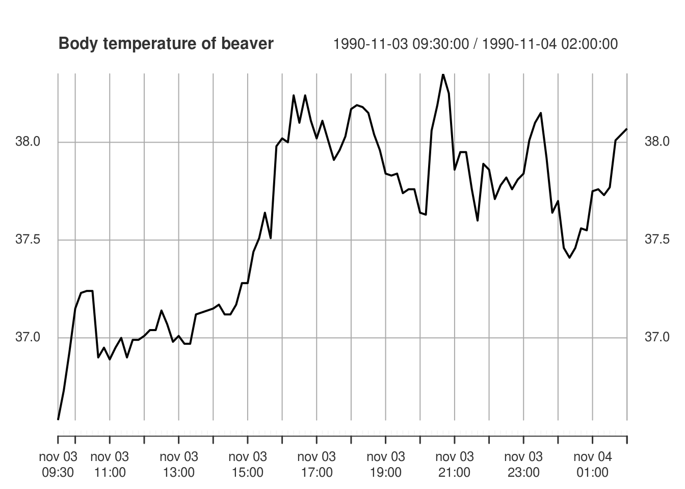

# Vanilla ts - works ok for regular time series
temp <- ts(beav2[, "temp"], start = 9.5, frequency = 6)
plot(temp, main = "Body temperature of beaver", ylab = "Temperature (in degree Celcius)")
lin_mod <- lm(temp ~ as.factor(activ), data = beav2)
lines(beav2[, "hours"], fitted(lin_mod), col = "blue")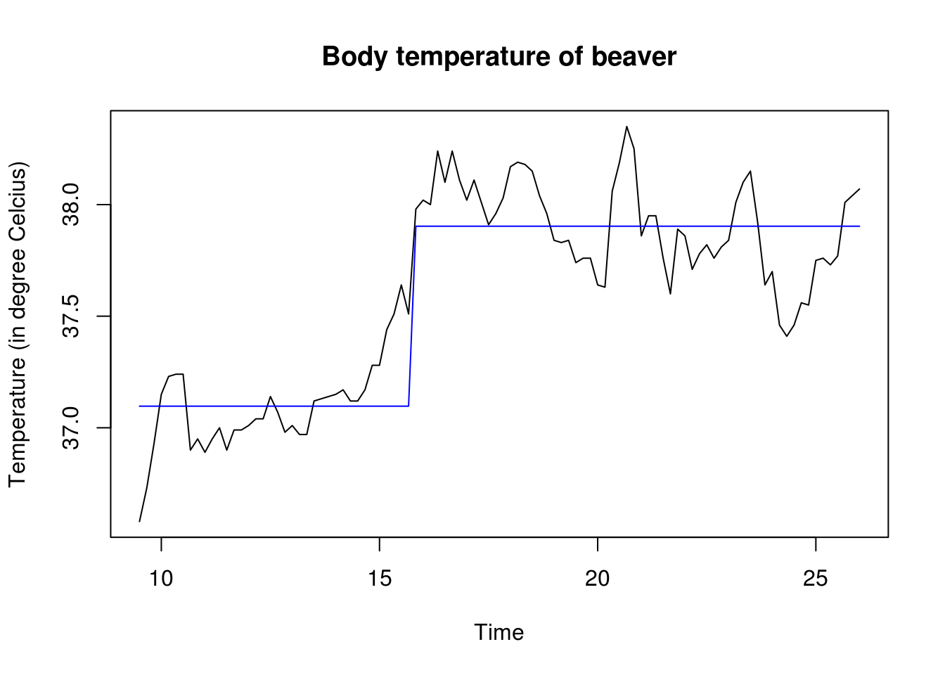

# Some trend remaining in the first part, before time

plot(residuals(lin_mod), ylab = "Residuals", main = "Residuals of linear model with simple change-point")
abline(h = 0)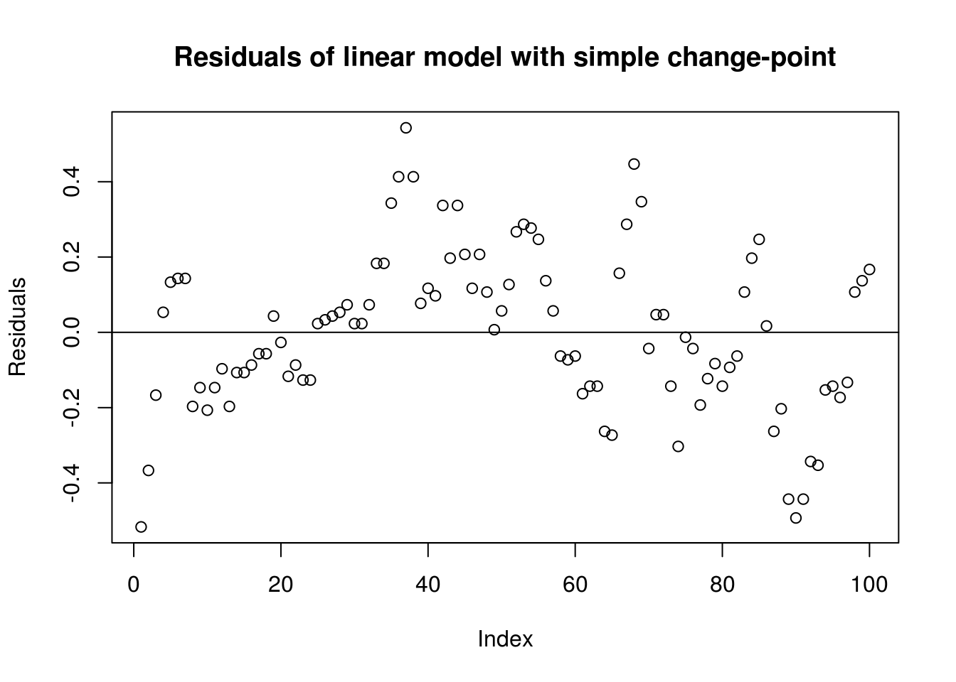

# Q-Q plot (1) with output from lm
plot(lin_mod, which = 2)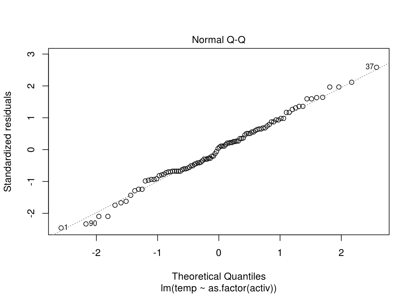

# (2) with qqnorm and tentative line with quartiles
qqnorm(residuals(lin_mod))
qqline(residuals(lin_mod))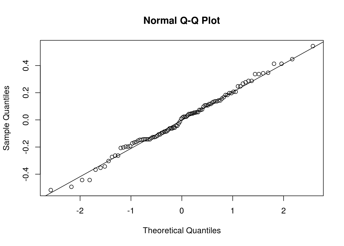

# (3) standardized manually
res <- residuals(lin_mod)
plot(qnorm(rank(res)/(length(res) + 1)), res/sd(res), pty = "s", bty = "l", 
    xlab = "Theoretical Quantiles", ylab = "Sample Quantiles", main = "Normal Q-Q plot", 
    pch = 20, col = rgb(0, 0, 0, 0.5))
abline(a = 0, b = 1)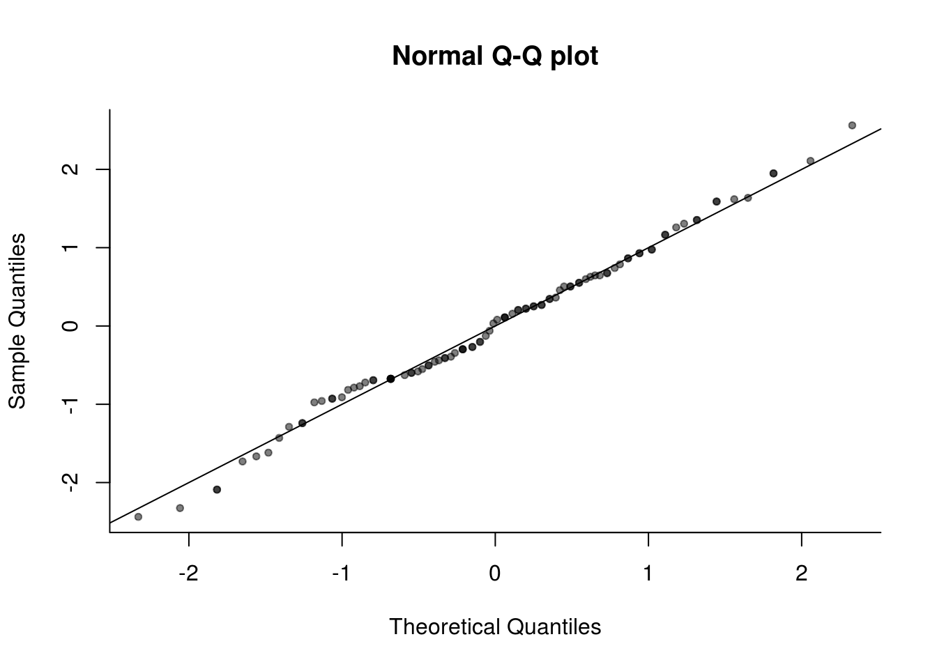

plot(res[-length(res)], res[-1], xlab = expression(Y[t - 1]), ylab = expression(Y[t]), 
    main = "Lagged residuals")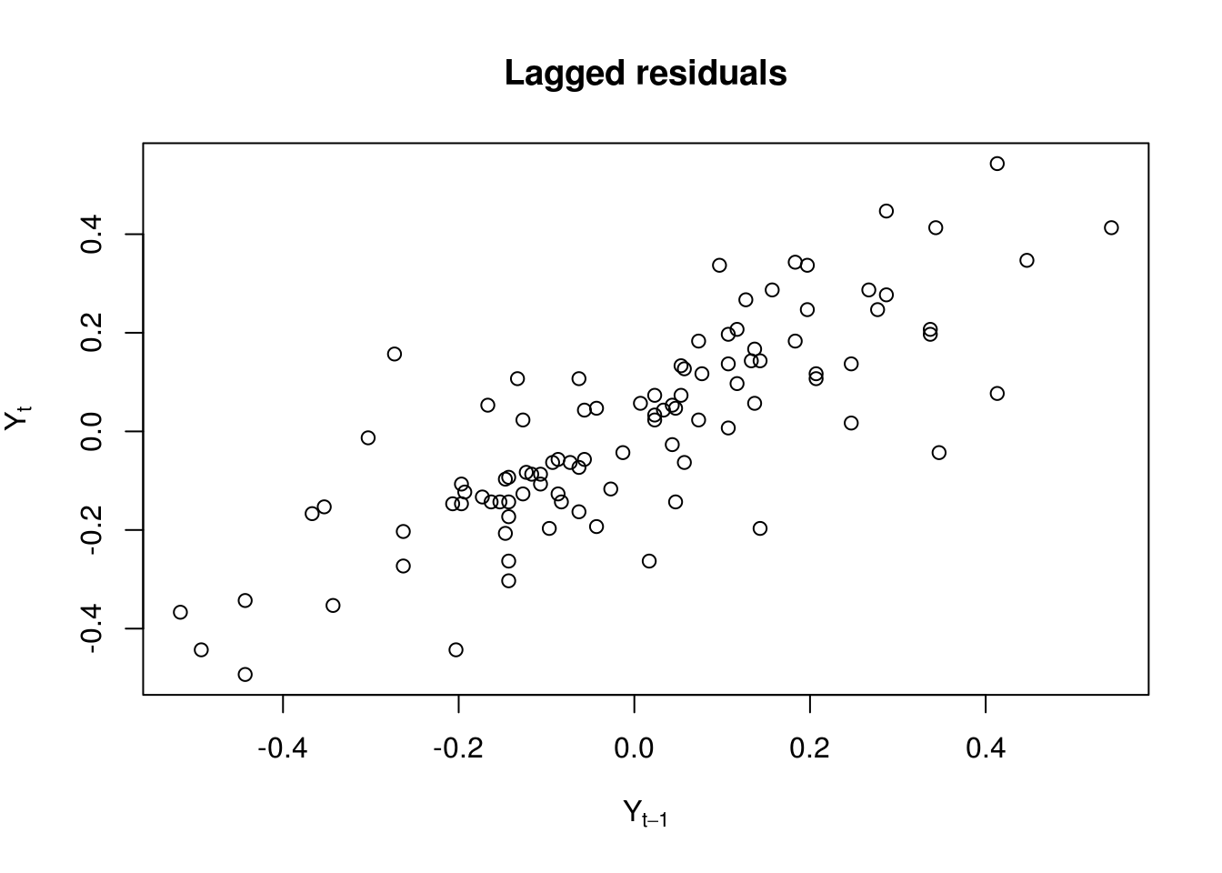

1.7.2 Solutions 2: SP500 daily returns

Download the dataset using the following command
Obtain the daily percent return series and plot the latter against time.
With the help of graphs, discuss evidences of seasonality and nonstationarity. Are there seasons of returns?
Plot the (partial) correlogram of both the raw and the return series. Try the acf with na.action=na.pass and without (by e.g. converting the series to a vector using as.vector. Comment on the impact of ignoring time stamps.
Plot the (partial) correlogram of the absolute value of the return series and of the squared return series. What do you see?

sp500 <- tseries::get.hist.quote(instrument = "^GSPC", start = "2000-01-01", 
    end = "2016-12-31", quote = "AdjClose", provider = "yahoo", origin = "1970-01-01", 
    compression = "d", retclass = "zoo")

time series starts 2000-01-03
time series ends   2016-12-30

library(xts)
library(lubridate)
# Daily return in percentage
spret <- 100 * diff(log(sp500))
plot(spret, ylab = "Daily returns (%)", main = "Percentage daily returns of the SP-500")
# local trend to see if there is any evidence of non-zero trend
lines(index(spret), lowess(spret, f = 1/5)$y, col = 2, lwd = 2)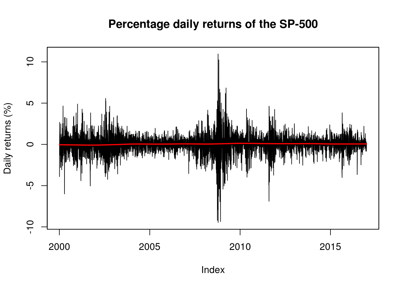

# Volatility as function of month
plot(jitter(month(spret), amount = 1/3), spret, pch = 20, ylab = "Daily percent returns", 
    xlab = "Month", bty = "l")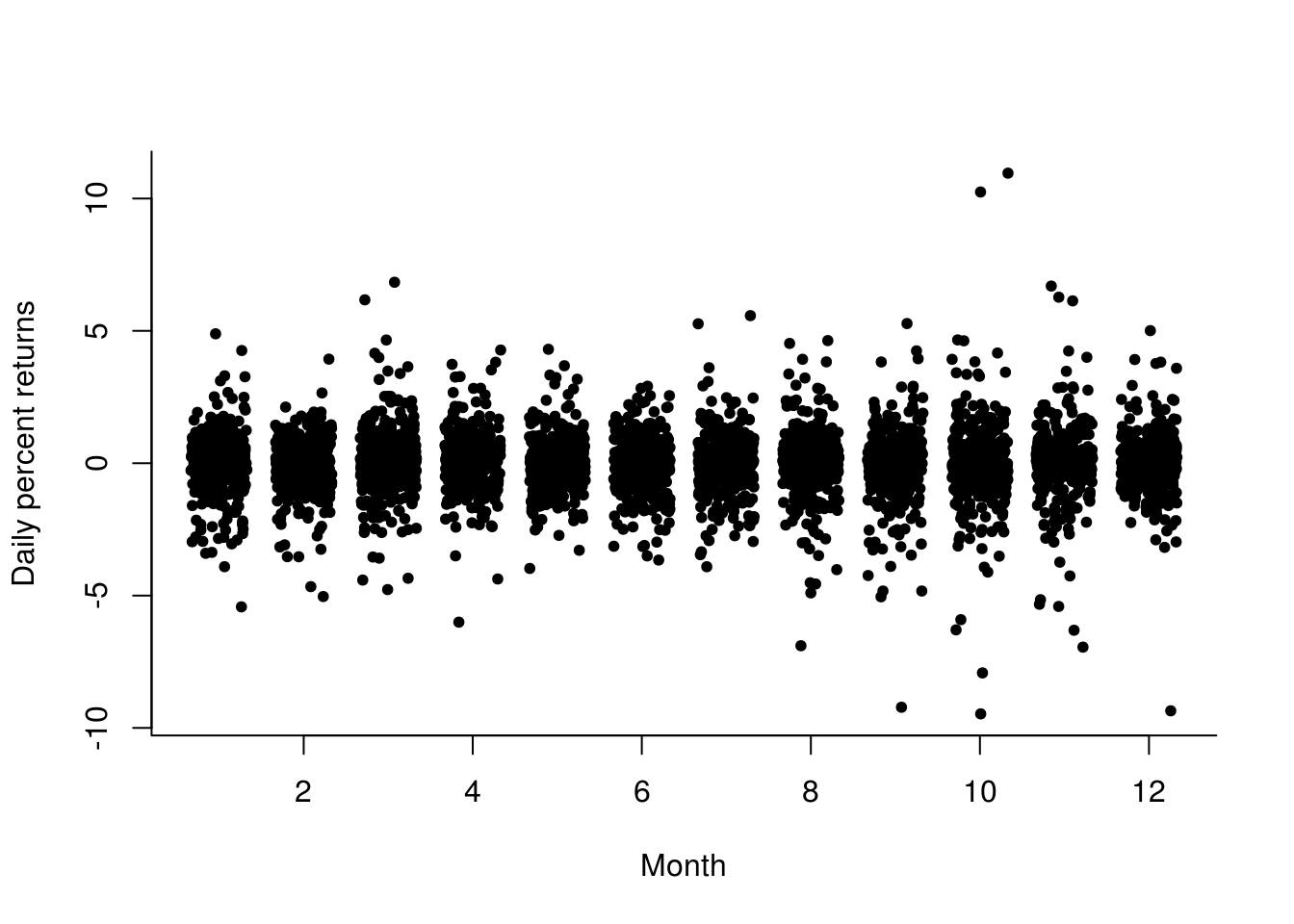

boxplot(as.vector(spret) ~ factor(wday(spret), labels = c("Mon", "Tue", "Wed", 
    "Thu", "Fri")), xlab = "Day of the week", pch = 20, col = rgb(0, 0, 0, 0.4), 
    ylab = "Daily percent returns", bty = "l")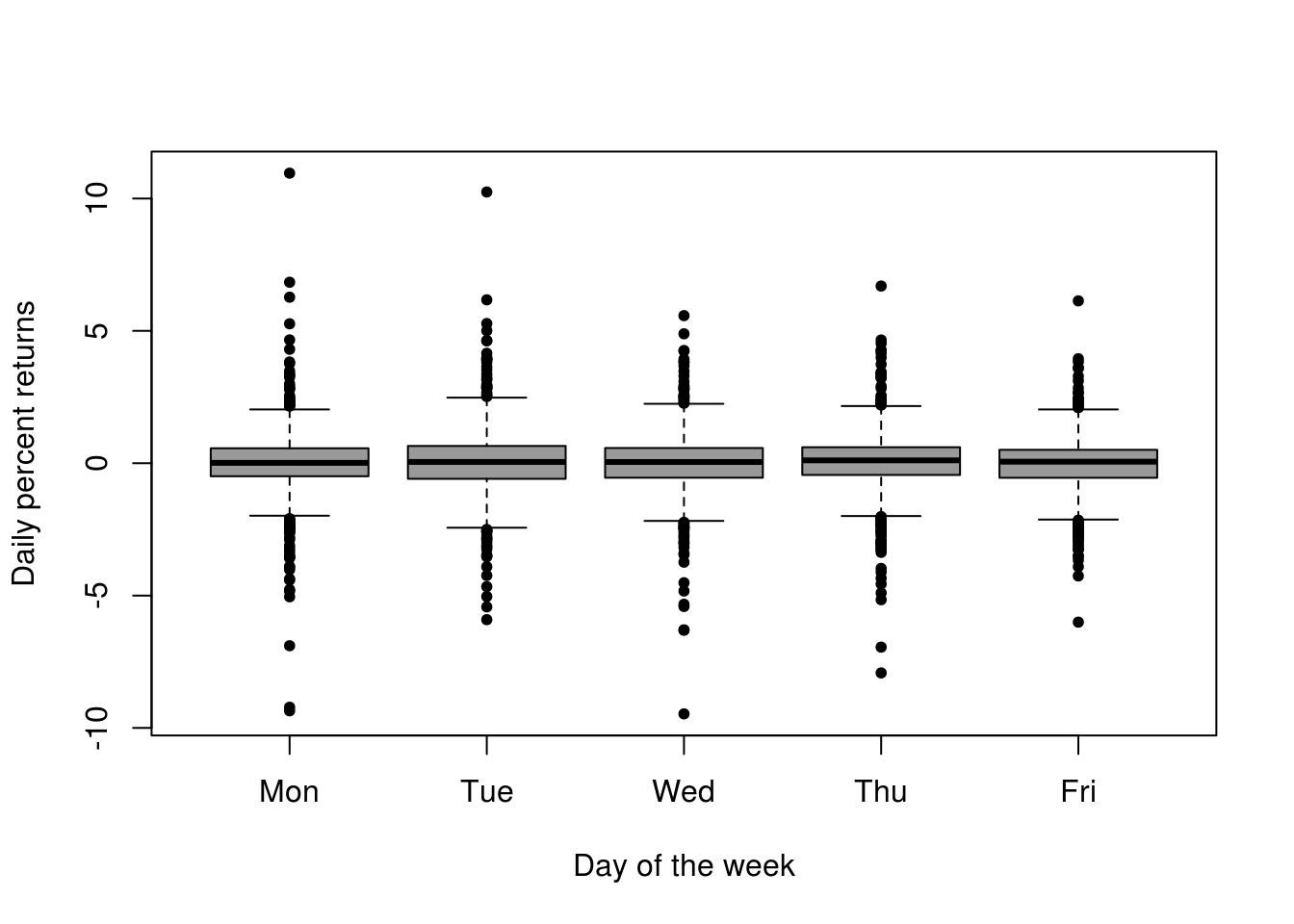

# More uncertainty in March-May and August-November Some more extremes early
# in the week

par(mfrow = c(1, 2))
title_sp <- "Daily return of \nadjusted SP500 at closure"
TSA::acf(spret, na.action = na.pass, main = title_sp)
TSA::acf(na.omit(as.vector(spret)), main = title_sp)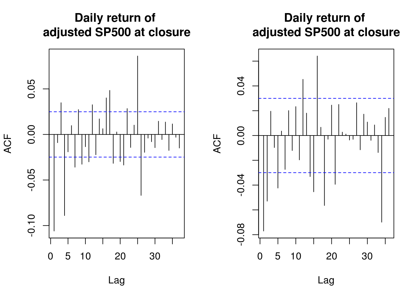

dev.off()

null device 
          1

pacf(spret, na.action = na.pass, main = title_sp)

# (P)ACF of absolute value of daily returns
TSA::acf(abs(spret), na.action = na.pass, main = title_sp)
pacf(abs(spret), na.action = na.pass, main = title_sp)
# (P)ACF of squared daily returns
TSA::acf(I(spret^2), na.action = na.pass, main = title_sp)
pacf(I(spret^2), na.action = na.pass, main = title_sp)

1.7.3 Solutions 3: Simulated data

The first 5 parts of the question are straightforward and left to the reader.

Simulate 500 observations from an AR(1) process with parameter values \(\alpha \in \{0.1, 0.5, 0.9, 0.99\}\).
Repeat for MA processes of different orders. There is no restriction on the coefficients of the latter for stationarity, unlike the AR process.
Sample from an ARCH(1) process with Gaussian innovations and an ARCH(1) process with Student-\(t\) innovations with df=4. Look at the correlogram of the absolute residuals and the squared residuals.
The dataset EuStockMarkets contains the daily closing prices of major European stock indices. Type ?EuStockMarkets for more details and plot(EuStockMarkets) to plot the four series (DAX, SMI, CAC and FTSE). Use plot(ftse <- EuStockMarkets[,"FTSE"]) to plot the FTSE series and plot(100*diff(log(ftse))) to plot its daily log return. Play with the ARCH simulation functions to generate some similar processes.
Simulate a white noise series with trend \(t\) and \(\cos(t)\), of the form \(X_t=M_t+S_t+Z_t\), where \(Z_t \sim \mathsf{N}(0,\sigma^2)\) for different values of \(\sigma^2\). Analyze the log-periodogram and the (partial) correlograms. What happens if you forget to remove the trend?
Do the same for multiplicative model with lognormal margins, with structure \(X_t=M_tS_tZ_t\).
For steps 5 and 6, plot the series and test the assumptions that they are white noise using the Ljung-Box test. Note you need to adjust the degrees of freedom when working with residuals from e.g. ARMA models.

n <- 100
tim <- scale(1:n)
x <- 5 * tim + cos(2 * pi * tim/n) + rnorm(n, sd = 3)
plot(x, type = "l", main = "Simulated series with seasonality and trend")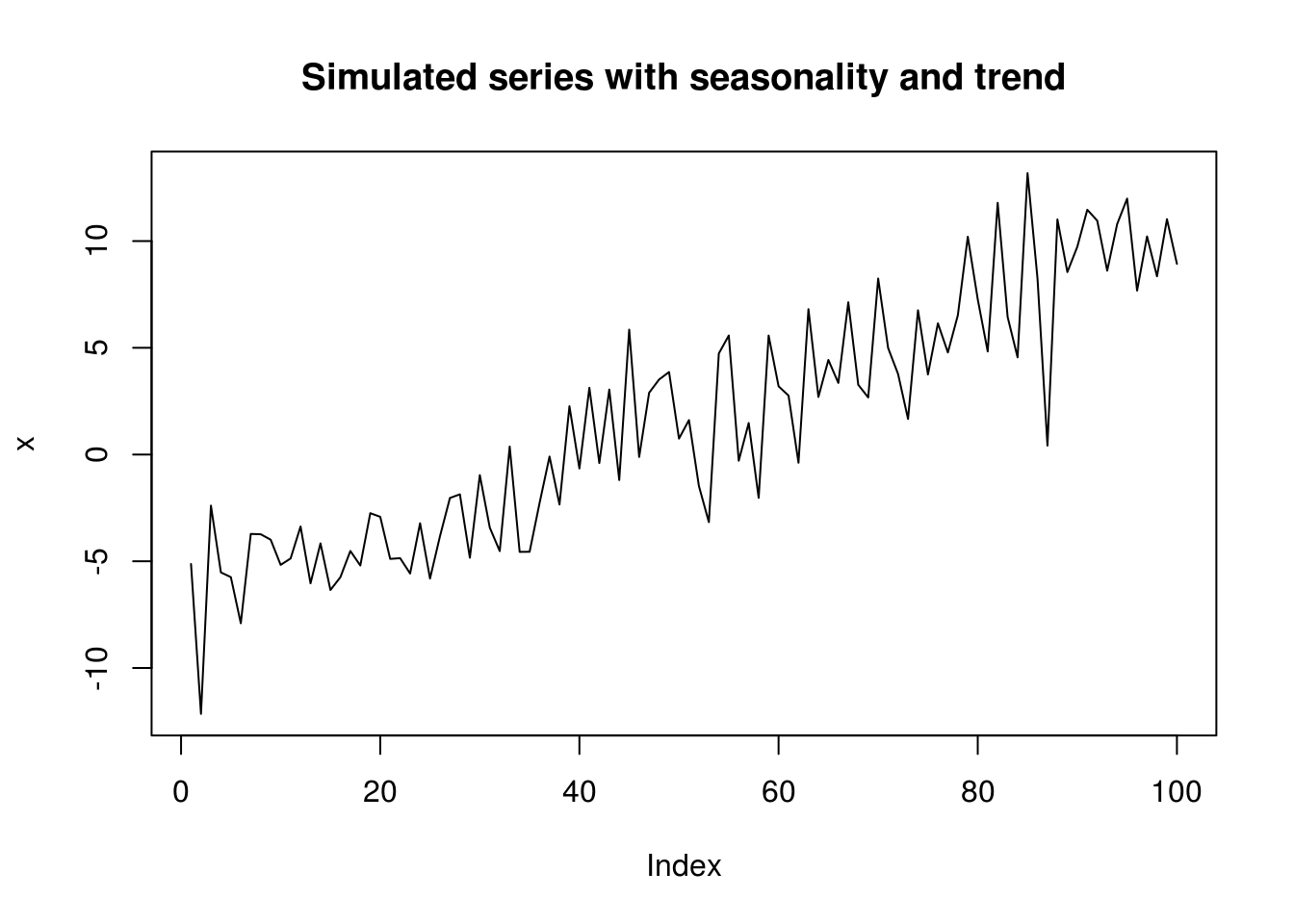

Box.test(x, type = "L")


    Box-Ljung test

data:  x
X-squared = 61.616, df = 1, p-value = 4.219e-15

par(mfrow = c(1, 3))  # plots side by side
TSA::acf(x, main = "Simulated series")
pacf(x, main = "Simulated series")
spectrum(x, main = "Simulated series")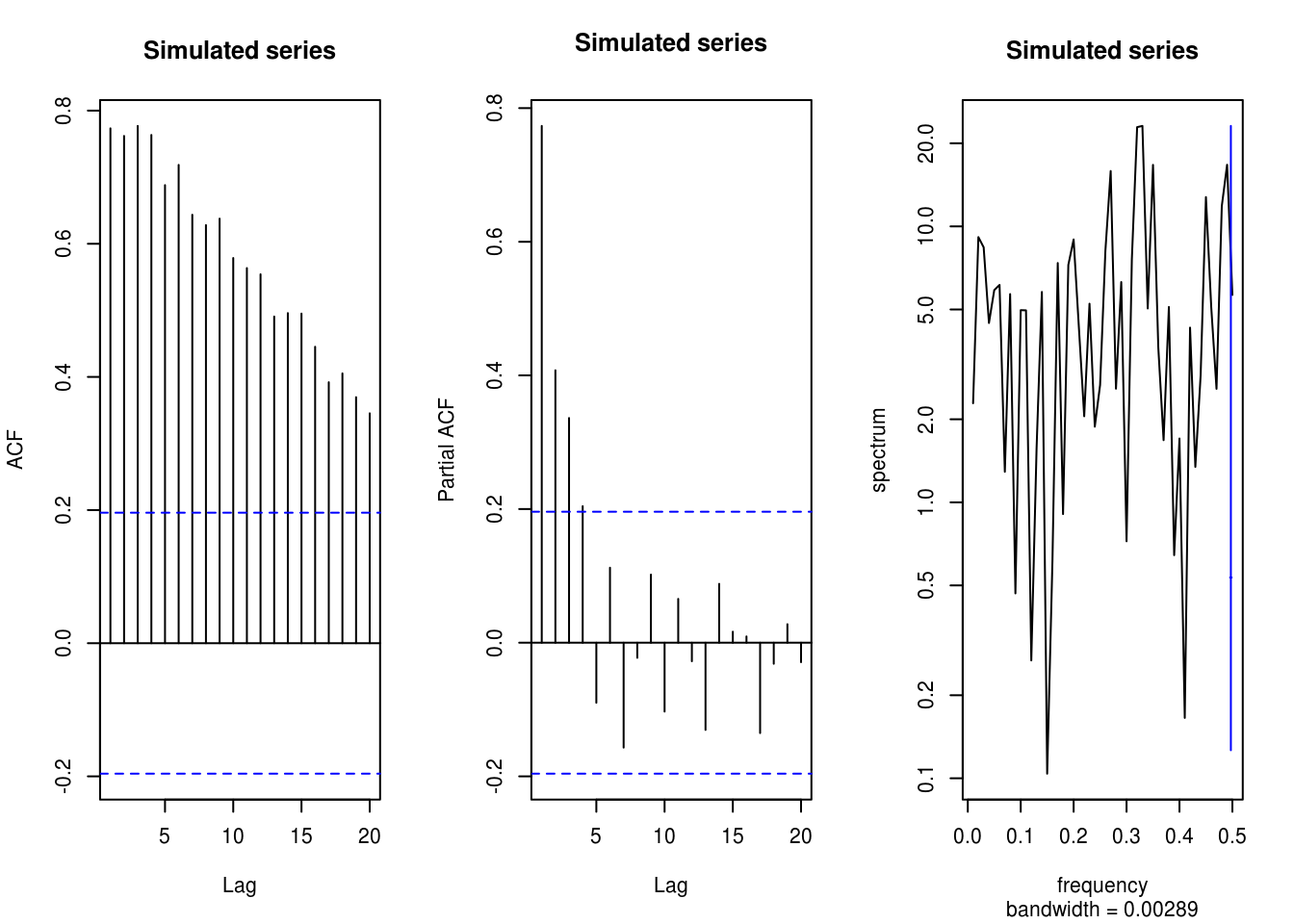

# Nothing in spectrum, persistence in the (p)acf
x <- 5 * tim + cos(2 * pi * tim/n) + rnorm(n, sd = 0.5)
TSA::acf(x, main = "Simulated series")
pacf(x, main = "Simulated series")
spectrum(x, main = "Simulated series")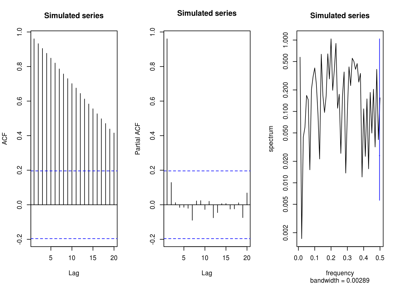

# Worst if the signal is strong relative to noise

y <- residuals(lm(x ~ 1 + tim))
TSA::acf(y, main = "Detrended series")
pacf(x, main = "Detrended series")
spectrum(y, main = "Detrended series")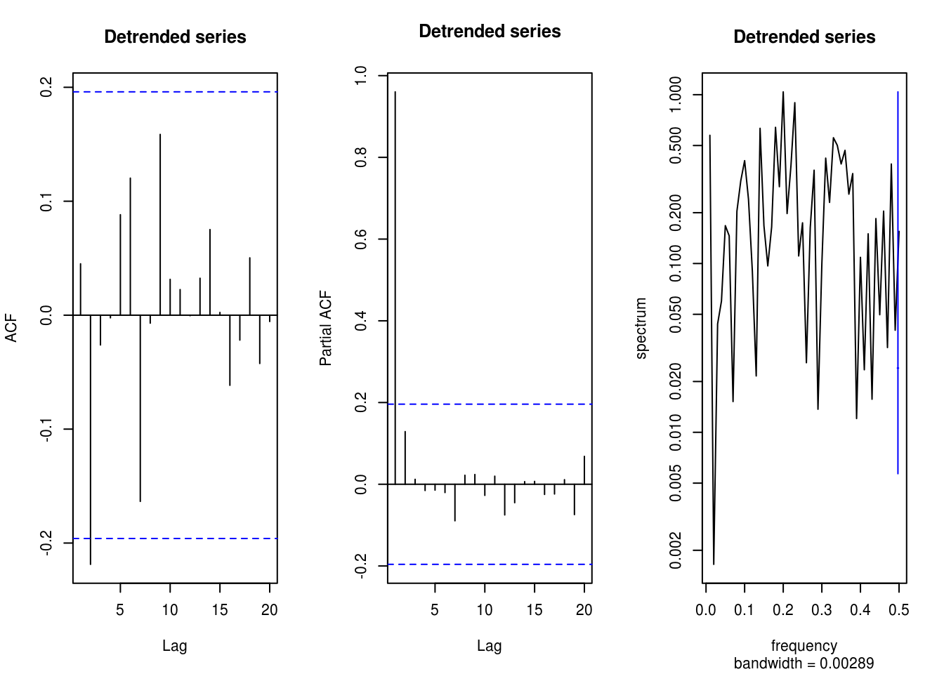

# The cosine still induces some lag-one dependence in pacf
plot(1:10, sapply(1:10, function(i) {
    Box.test(y, lag = i, type = "Ljung", fitdf = min(i - 1, 2))$p.value
}), ylab = "P-value", xlab = "lag")
# These low p-values at large lags are due to the cosine term

mult <- exp(scale(x))
TSA::acf(mult, main = "Multiplicative series")
pacf(mult, main = "Multiplicative series")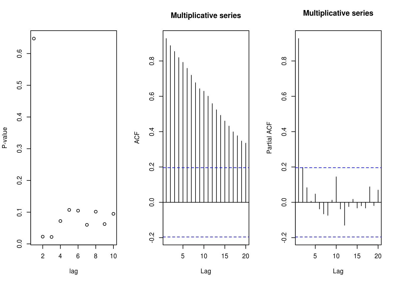

spectrum(mult, main = "Multiplicative series")
Box.test(mult, type = "L")


    Box-Ljung test

data:  mult
X-squared = 88.489, df = 1, p-value < 2.2e-16

graphics.off()
# Now large impact on spectrum, and nonlinear features!
plot(mult, main = "Multiplicative series with lognormal margins", ylab = "", 
    xlab = "Time")
# Note that decompose has an option type='multiplicative' for seasonal
# components

1.7.4 Solutions 4: Mauna Loa Atmospheric CO₂ Concentration

Load and plot the CO₂ dataset from NOAA. Pay special attention to the format, missing values, the handling of string and the description. Use ?read.table for help, and look carefully at arguments file, sep, na.strings, skip and stringsAsFactors. From now on, we will work with the complete series (termed interpolated in the description).
Try removing the trend using a linear model. Plot the residuals against month of the year.
Remove the trend and the periodicity with a Fourier basis (with period 12). Be sure to include both sin and cos terms together. Recall that the standard Wald tests for the coefficients is not valid in the presence of autocorrelation! You could also use poly or splines::bs to fit polynomials or splines to your series.
Plot the lagged residuals. Are there evidence of correlation?
Use the function filter to smooth the series using a 12 period moving average.
Inspect the spectrum of the raw series and of the smoothed version.
Inspect the spectrum of the detrended raw series.
Test for stationarity of the deseasonalized and detrended residuals using the KPSS test viz. tseries::kpss.test.
Use the decompose and the stl functions to obtain residuals.
Plot the (partial) correlogram for both decomposition and compare them with the output of the linear model.

# Because of comment.char=#, all the first lines are skipped But we lose the
# header
co2 <- read.table(file = "ftp://aftp.cmdl.noaa.gov/products/trends/co2/co2_mm_mlo.txt", 
    na.strings = "-99.99", stringsAsFactors = FALSE, col.names = c("year", "month", 
        "time", "average", "interpolated", "trend", "monthly_mean"))
# install.packages('stlplus') #this package offers a version of stl that
# deals with NAs

ycap <- expression(paste("Monthly mean ", CO[2], " mole fraction (ppm)"))
mcap <- "Average monthly mean CO2 concentration\n determined from daily averages"
lin_mod <- lm(data = co2, interpolated ~ time)
with(co2, plot(interpolated ~ time, type = "l", xlab = "Time", bty = "l", ylab = ycap, 
    main = mcap))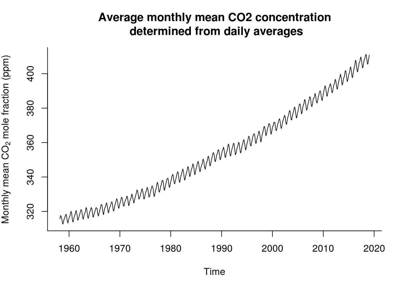

plot(co2$time, residuals(lin_mod), ylab = "Residual from `lm` (linear trend)", 
    xlab = "Time", main = mcap)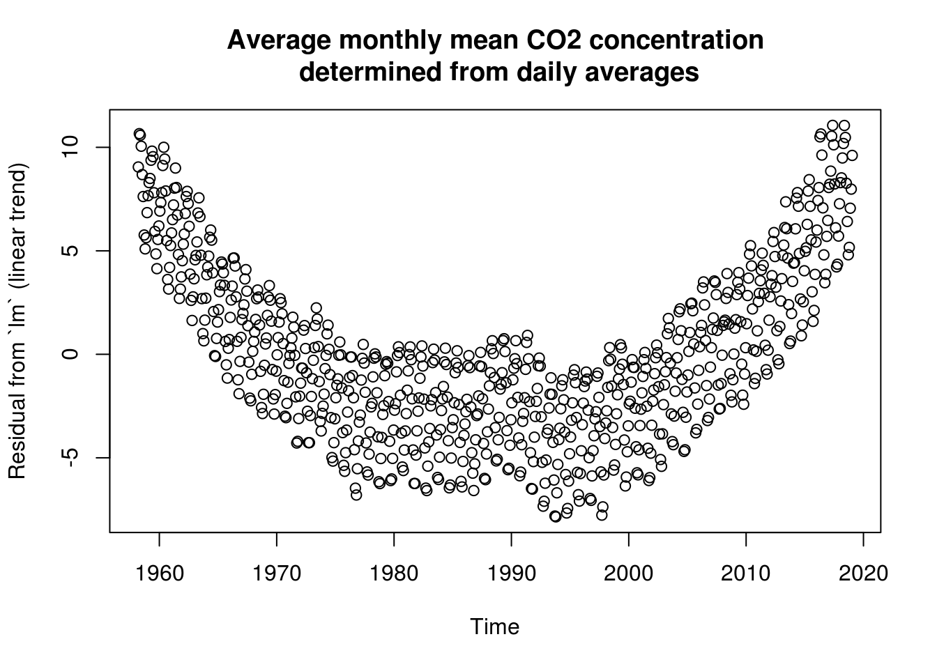

lin_mod <- update(lin_mod, . ~ . + I(time^2))
# same as lm(data=co2, interpolated ~ poly(time, degree = 2))
plot(co2$time, residuals(lin_mod), main = mcap, ylab = "Residual from `lm` (quadratic trend)", 
    xlab = "Time")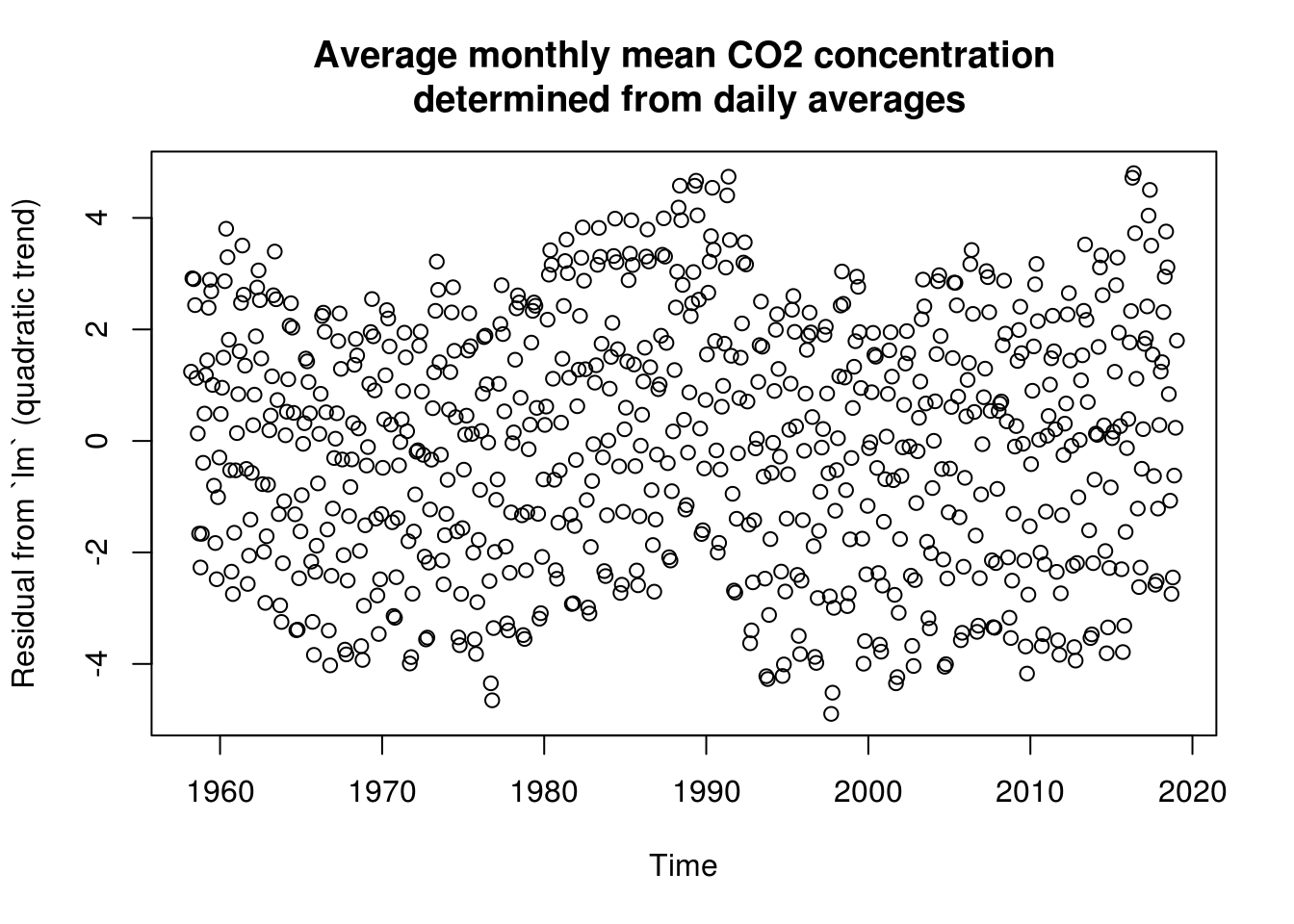

# Cast the full time series into a ts object
co2_ts <- with(co2, ts(data = interpolated, start = c(year[1], month[1]), end = c(tail(year, 
    1), tail(month, 1)), frequency = 12))
with(co2, plot(jitter(month, 1/3), residuals(lin_mod), ylab = "Residuals", xlab = "Month of year", 
    main = mcap))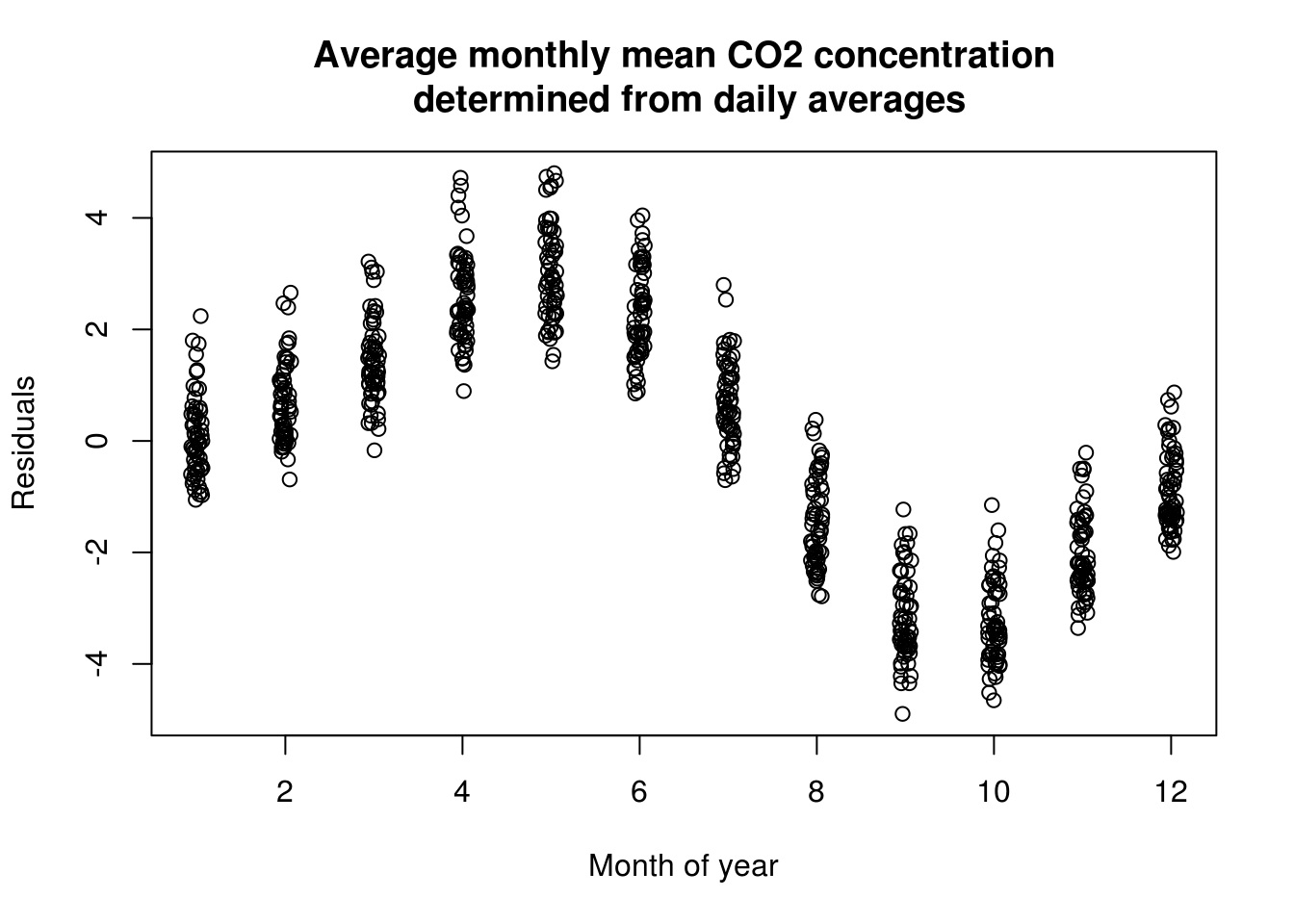

# Could create the basis manually
f_bs <- with(co2, fda::fourier(month, nbasis = 4, period = 12))[, -1]
lin_mod <- with(co2, lm(interpolated ~ splines::bs(time, df = 5, degree = 3) + 
    f_bs))
# summary(lin_mod) Is there structure left in the residuals?
plot(co2$time, residuals(lin_mod), ylab = "Residuals from final `lm` model", 
    xlab = "Time", main = mcap)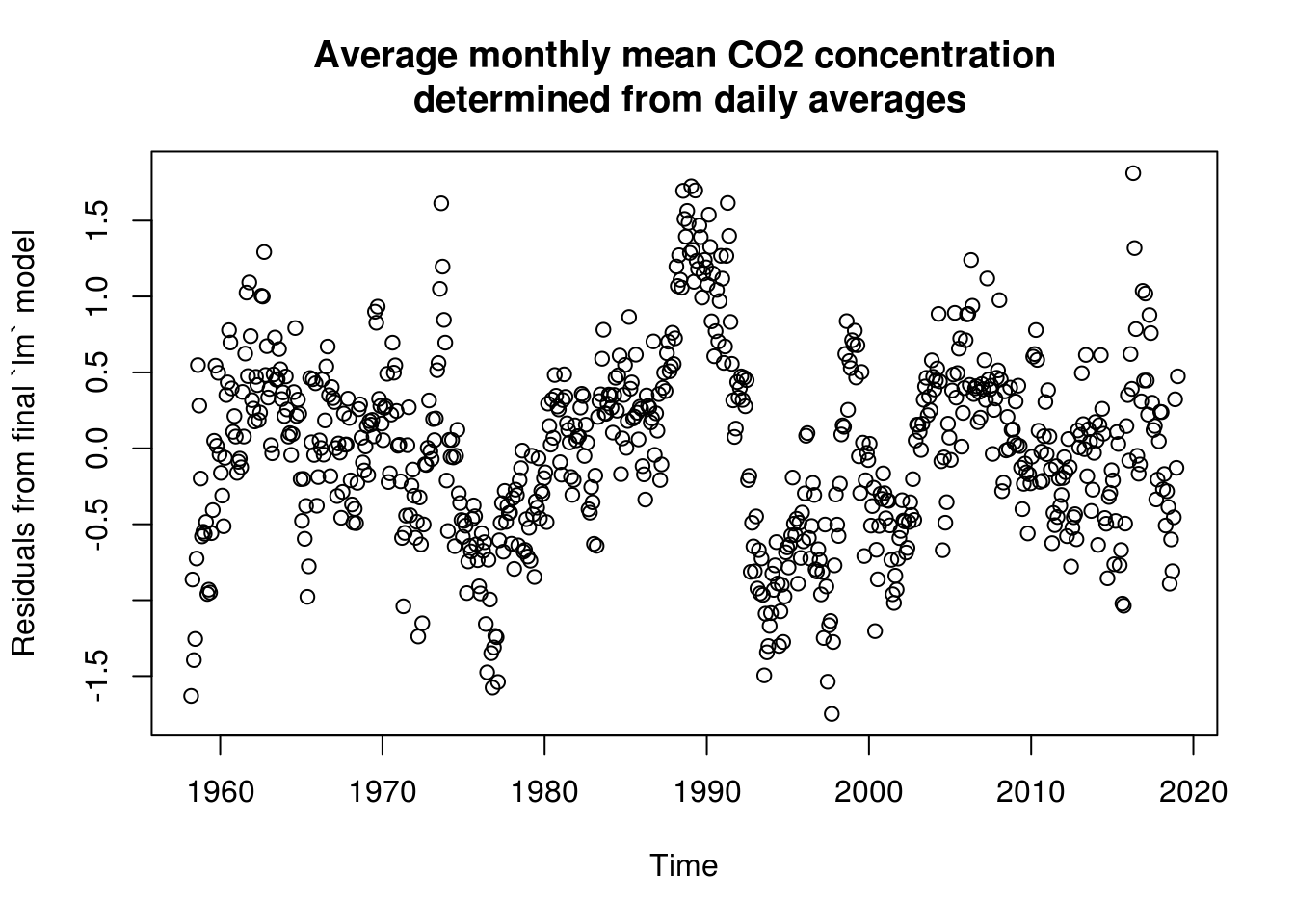

plot(co2$time, fitted(lin_mod), type = "l", ylab = ycap, main = mcap, bty = "l")
with(co2, lines(time, interpolated, col = 2))
legend(x = "topleft", legend = c("fitted", "data"), col = c(1, 2), lty = c(1, 
    1), bty = "n")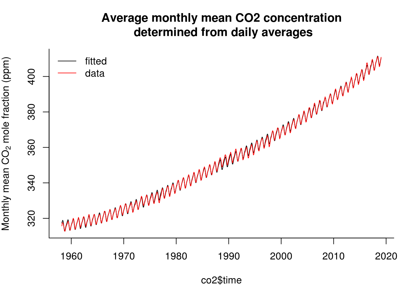

# Trend not quite adequate because more exponential growth.  The trend does
# poorly in low-high observations Some discrepancy between the frequencies
# and the fitted Creates residual harmonic patterns - because trend minus
# fitted
res <- residuals(lin_mod)

pairs.ts <- function(d, lag.max = 10) {
    old_par <- par(no.readonly = TRUE)
    n <- length(d)
    X <- matrix(NA, n - lag.max, lag.max)
    col.names <- paste("Time+", 1:lag.max)
    for (i in 1:lag.max) X[, i] <- d[i - 1 + 1:(n - lag.max)]
    par(mfrow = c(3, 3), pty = "s", mar = c(3, 4, 0.5, 0.5))
    lims <- range(X)
    for (i in 2:lag.max) plot(X[, 1], X[, i], panel.first = {
        abline(0, 1, col = "grey")
    }, xlab = "Time", ylab = col.names[i - 1], xlim = lims, ylim = lims, pch = 20, 
        col = rgb(0, 0, 0, 0.25))
    par(old_par)
}
pairs.ts(res)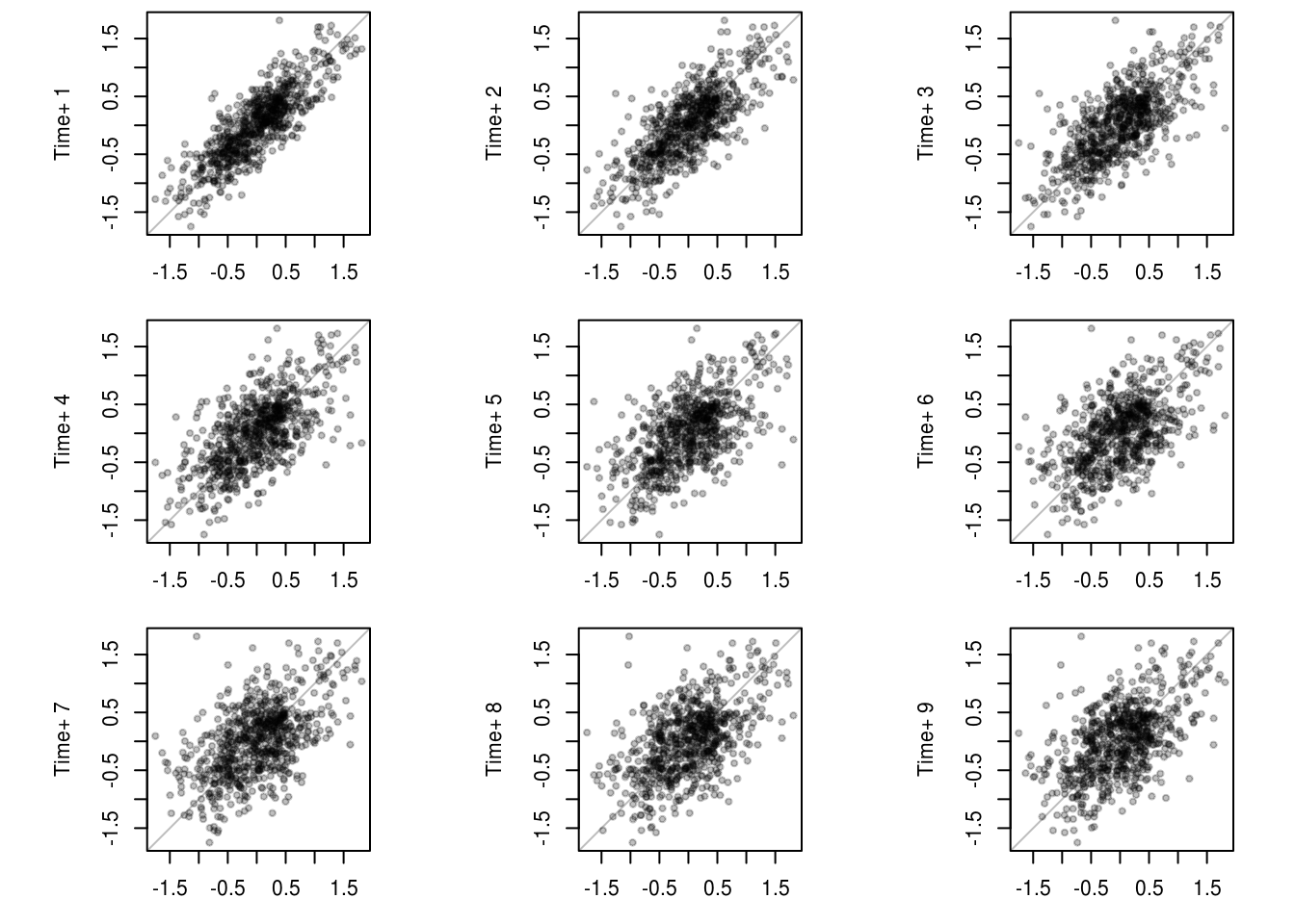

par(mfrow = c(1, 2))
TSA::acf(res, main = "Residuals")
pacf(res, main = "Residuals")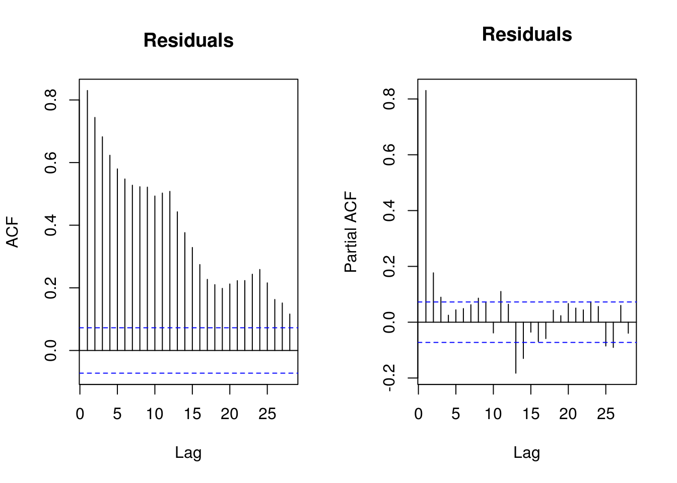

par(mfrow = c(1, 1))
# KS test: are residuals white noise?
cpgram(res, main = "Cumulative periodogram")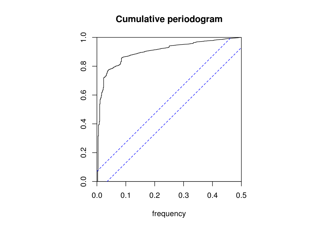

# No, as one would expect

# Spectrum of raw series
spectrum(co2$interpolated)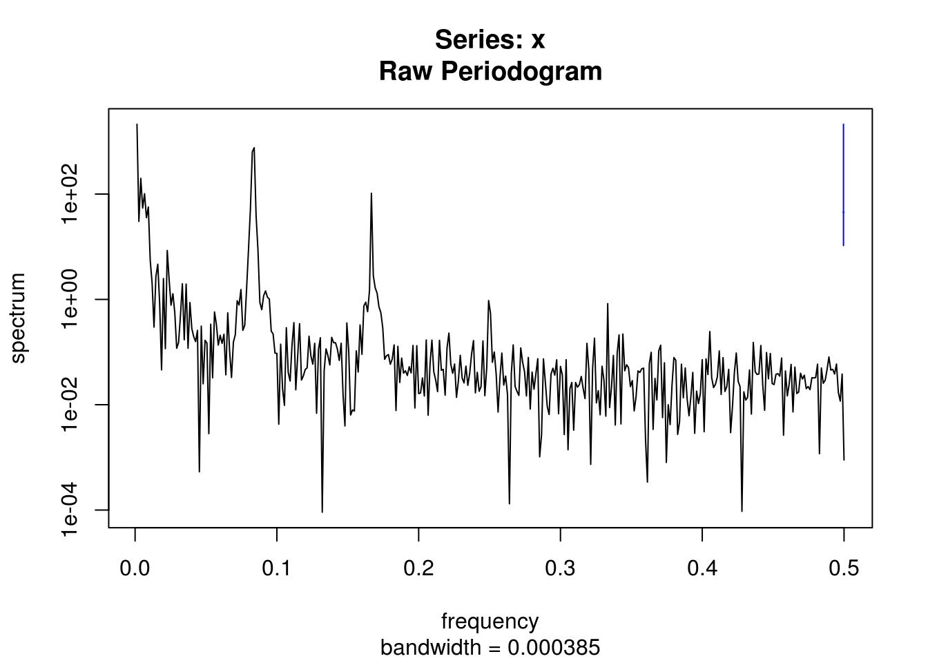

# default with vector is to have frequency on [0,0.5]
spectrum(co2_ts)  #otherwise corresponds to frequency of `ts`, here yearly

filtered <- filter(co2$interpolated, method = "convolution", filter = rep(1/12, 
    12))
spectrum(na.contiguous(filtered))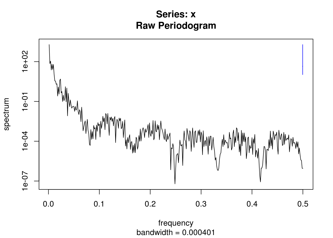

# Detrended smoothed series
spectrum(resid(lm(filtered ~ poly(co2$time, 2))))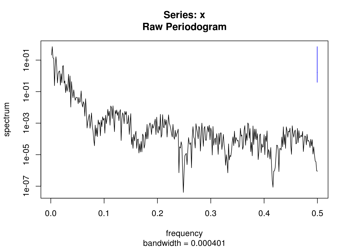

# Test for H0
`?`(tseries::kpss.test)
tseries::kpss.test(res, null = "Level")


    KPSS Test for Level Stationarity

data:  res
KPSS Level = 0.16743, Truncation lag parameter = 6, p-value = 0.1

# Fail to reject null that it is level stationary
tseries::kpss.test(res, null = "Trend")


    KPSS Test for Trend Stationarity

data:  res
KPSS Trend = 0.16743, Truncation lag parameter = 6, p-value =
0.03214

# Reject null at 5% that it is trend stationary

res_dec <- decompose(co2_ts)$random
res_stl <- stl(co2_ts, s.window = "periodic")$time.series[, "remainder"]

par(mfrow = c(1, 2))
# Some structure left due to incorrect model specification Residual
# frequency at lag 12-24 and two lag residuals
TSA::acf(res, na.action = na.pass, main = "Residuals from\n `lm`")
pacf(res, na.action = na.pass, main = "Residuals from\n `lm`")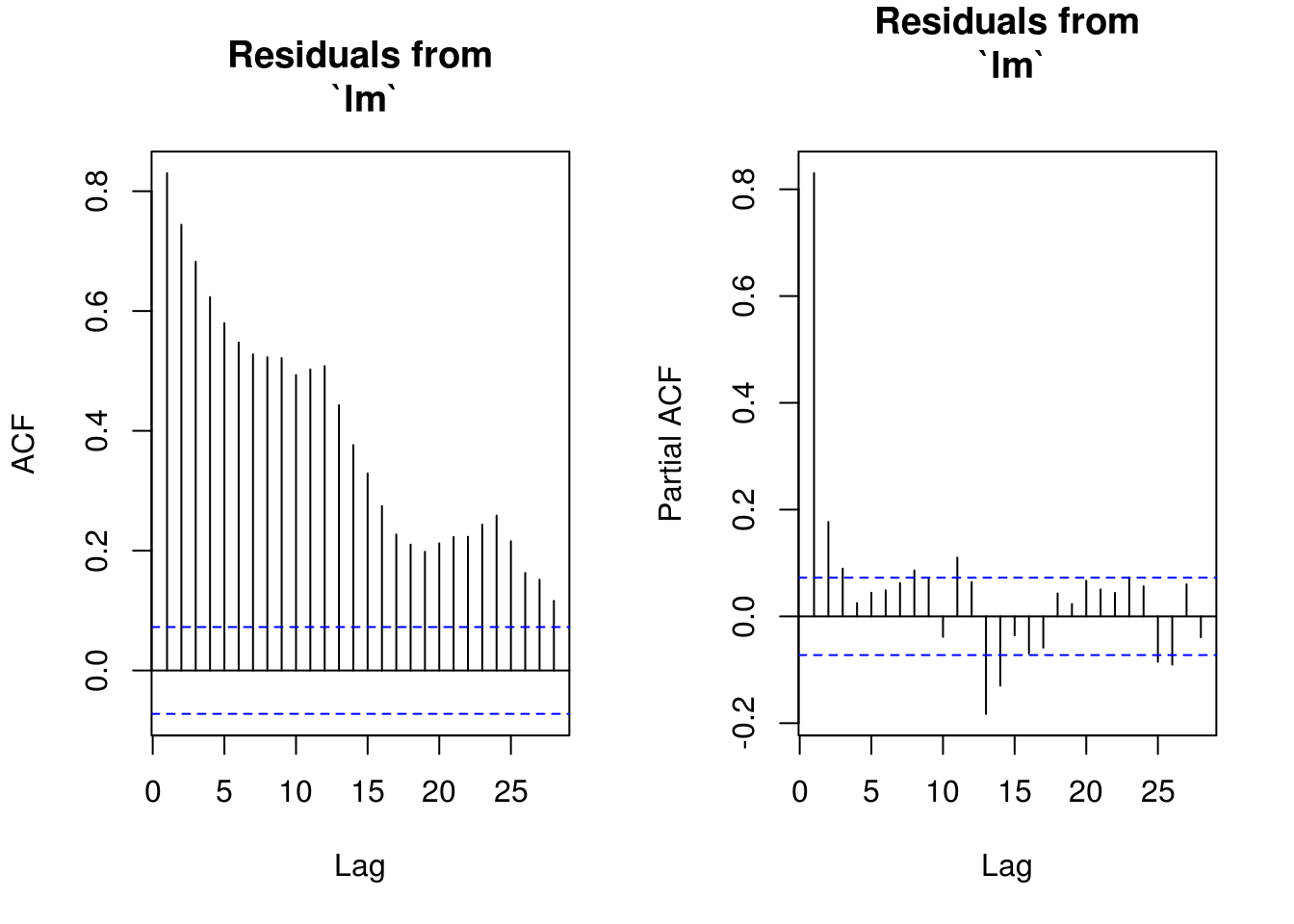

# Residuals show some remaining periodicity at year 1. Would need AR(1)
# model
TSA::acf(res_dec, na.action = na.pass, main = "Residuals from\n `decompose`")
pacf(res_dec, na.action = na.pass, main = "Residuals from\n `decompose`")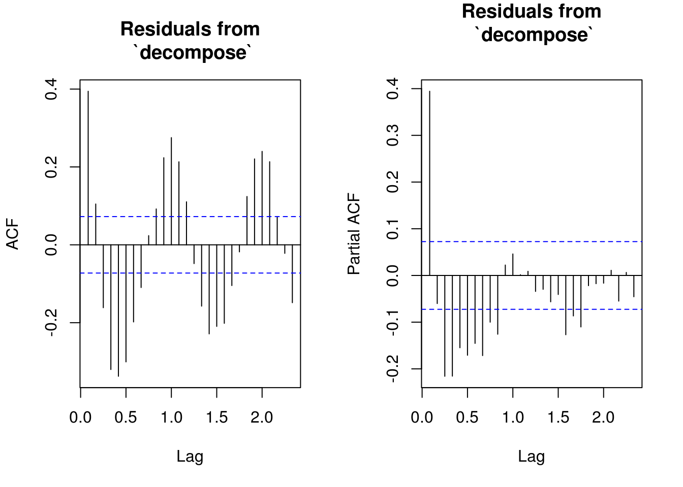

# Similar output
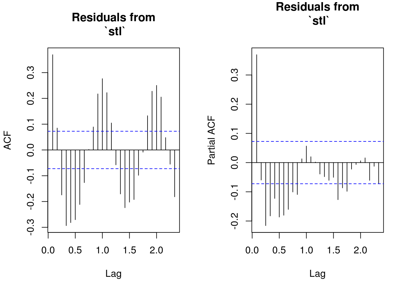
TSA::acf(res_stl, main = "Residuals from\n `stl`")
pacf(res_stl, main = "Residuals from\n `stl`")

1.7 Solutions to Exercises

1.7.1 Solutions 1: Beaver temperature

1.7.2 Solutions 2: SP500 daily returns

1.7.3 Solutions 3: Simulated data

1.7.4 Solutions 4: Mauna Loa Atmospheric CO2 Concentration

1.7.4 Solutions 4: Mauna Loa Atmospheric CO₂ Concentration