7 Computational strategies and diagnostics
The Bayesian workflow is a coherent framework for model formulation construction, inference and validation. It typically involves trying and comparing different models, adapting and modifying these models (Gelman et al. 2020); see also Michael Betancourt for excellent visualizations. In this chapter, we focus on three aspects of the workflow: model validation, evaluation and comparison.
Learning objectives:
At the end of the chapter, students should be able to
- use output of MCMC to obtain estimates and standard errors.
- choose suitable test statistics to evaluate model adequacy.
- assess convergence using graphical tools and effective sample size.
- perform model comparisons using Bayes factor or predictive measures.
- diagnose performance of MCMC algorithms (in terms of mixing and effective sample size).
- implement strategies to improve sampling performance, including block updates, reparametrization and marginalization.
We begin with a running example that will be used to illustrate the concepts.
Example 7.1 (Poisson random effect models) We consider data from an experimental study conducted at Tech3Lab on road safety. In Brodeur et al. (2021), 31 participants were asked to drive in a virtual environment; the number of road violation was measured for different type of distractions (phone notification, phone on speaker, texting and smartwatch). The data are balanced, with each participant exposed to each task exactly once.
We model the data using a Poisson mixed model to measure the number of violations, nviolation, with a fixed effect for task, which captures the type of distraction, and a random effect for participant id. The hierarchical model fitted for individual \(i\) \((i=1, \ldots, 34)\) and distraction type \(j\) \((j=1, \ldots, 4)\) is \[\begin{align*}
Y_{ij} &\sim \mathsf{Poisson}\{\mu_{ij} = \exp(\beta_{j} + \alpha_i)\},\\
\beta_j &\sim \mathsf{Gauss}(0, 100), \\
\alpha_i &\sim \mathsf{Gauss}(0, \kappa^2), \\
\kappa &\sim \mathsf{Student}_{+}(0,1,3).
\end{align*}\] so observations are conditionally independent given hyperparameters \(\boldsymbol{\alpha}\) and \(\boldsymbol{\beta}.\)
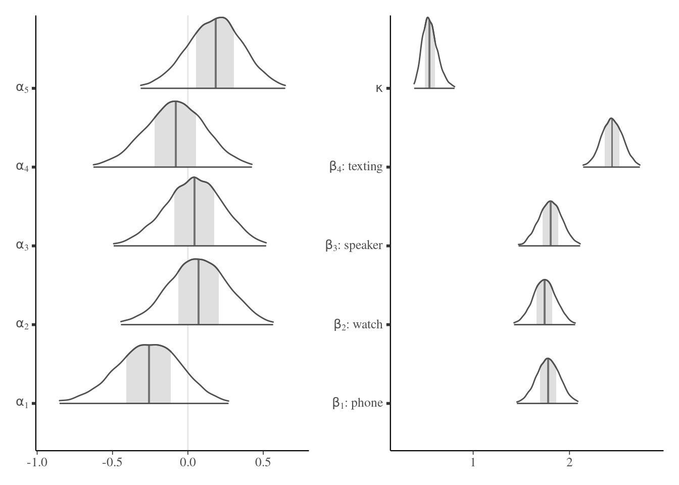
We can look at some of posterior distribution of the 31 random effects (here the first five individuals) and the fixed effect parameters \(\boldsymbol{\beta},\) plus the variance of the random effect \(\kappa\): there is strong evidence that the latter is non-zero, suggesting strong heterogeneity between individuals. The distraction which results in the largest number of violation is texting, while the other conditions all seem equally distracting on average (note that there is no control group with no distraction to compare with, so it is hard to draw conclusions).
Remark 7.1 (Bayesian random effect models). In frequentist statistics, there is a distinction made in mixed-effect models between parameters that are treated as constants, termed fixed effects and corresponding in this example to \(\boldsymbol{\beta},\) and random effects, equivalent to \(\boldsymbol{\alpha}.\) There is no such distinction in the Bayesian paradigm, except perhaps for the choice of prior and the informativeness of the latter.
7.1 Sensitivity analysis
Do priors matter? The answer to that question depends strongly on the model, and how much information the data provides about hyperparameters. While this question is easily answered in conjugate models (the relative weight of hyperparameters relative to data can be derived from the posterior parameters), it is not so simple in hierarchical models, where the interplay between prior distributions is often more intricate. To see the impact, one often has to rely on doing several analyses with different values fr the prior and see the sensitivity of the conclusions to these changes, for example by considering a vague prior or modifying the parameters values (say halving or doubling). If the changes are immaterial, then this provides reassurance that our analyses are robust.
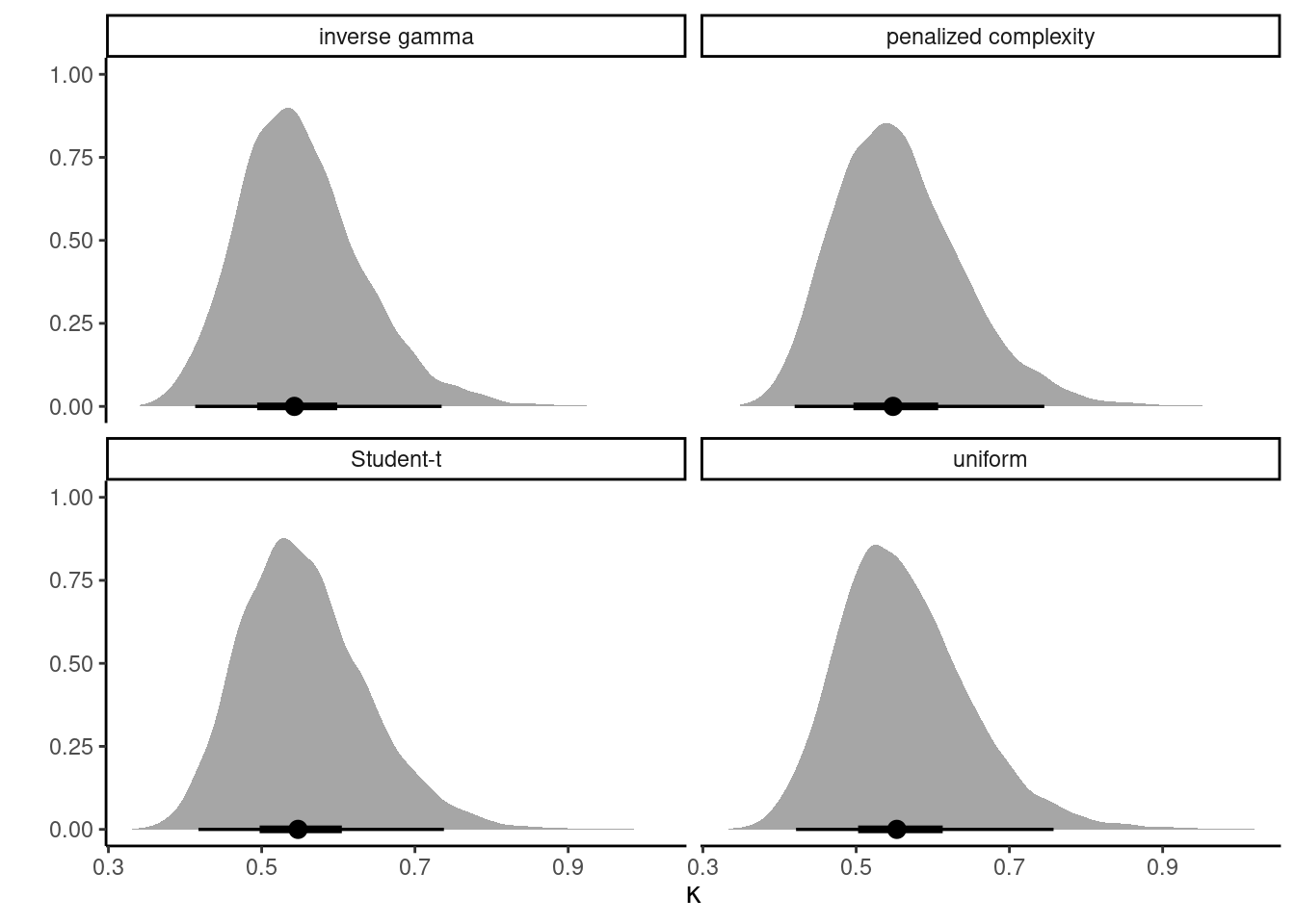
Example 7.2 To check the sensitivity of the conclusion, we revisit the modelling of the smartwatch experiment data using a Poisson regression and compare four priors: a uniform prior truncated to \([0, 10],\) an inverse gamma \(\mathsf{InvGamma}(0.01, 0.01)\) prior, a penalized complexity prior such that the 0.95 percentile of the scale is 5, corresponding to \(\mathsf{Exp}(0.6).\) Since each distraction type appears 31 times, there is plenty of information to reliably estimate the dispersion \(\kappa\) of the random effects \(\alpha\): the different density plots in Figure 7.2 are virtually indistinguishable from one another. This is perhaps unsurprising given the large number of replicates, and the significant variability between groups.
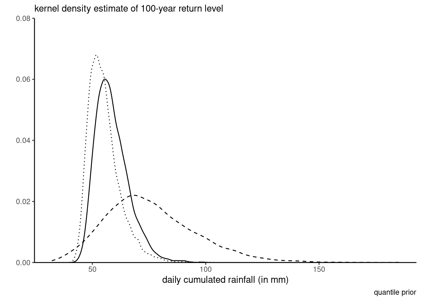
Example 7.3 (Extreme rainfall in Abisko, Sweden) As illustrating example, consider maximum daily cumulated rainfall in Abisko, Sweden. The time series spans from 1913 until December 2014; we compute the 102 yearly maximum, which range from 11mm to 62mm, and fit a generalized extreme value distribution to these.
For the priors, suppose an expert elicits quantiles of the 10, 50 and 100 years return levels; say 30mm, 45mm and 70mm, respectively, for the median and likewise 40mm, 70mm and 120mm for the 90% percentile of the return levels. We can compute the differences and calculate the parameters of the gamma distribution through moment-matching: this gives roughly a shape of \(\alpha_1=18.27\) and \(\beta_1=0.6,\) etc. Figure 7.3 shows the transfer from the prior predictive to the posterior distribution. The prior is much more dispersed and concentrated on the tail, which translates in a less peaked posterior than using a weakly informative prior (dotted line): the mode of the latter is slightly to the left and with lower density in the tail.
For a given problem, there are many different Markov chain Monte Carlo algorithms that one can implement: they will typically be distinguished based on the running time per iteration and the efficiency of the samplers, with algorithms providing realizations of Markov chains with lower autocorrelation being preferred. The purpose of this section is to review these in turn, and to go over tricks that can improve mixing.
–>
The target of inference is a functional (i.e., one-dimensional summaries of the chain): we need to have convergence of the latter, but also sufficient effective sample size for our averages to be accurate (at least to two significant digits).
To illustrate these, we revisit the model from Example 7.1 with a penalized complexity prior for the individual effect \(\alpha_i\) and vague normal priors. We also fit a simple Poisson model with only the fixed effect, taking \(Y_{ij} \sim \mathsf{Poisson}\{\exp(\beta_j)\}\) with \(\beta_j \sim \mathsf{Gauss}(0,100)\). This model has too little variability relative to the observations and fits poorly as is.
For the Poisson example, the effective sample size for the \(\boldsymbol{\beta}\) for the multilevel model is a bit higher than 1000 with \(B=5000\) iterations, whereas we have for the simple naive model is \(1.028\times 10^{4}\) for \(B=10000\) draws, suggesting superefficient sampling. The dependency between \(\boldsymbol{\alpha}\) and \(\boldsymbol{\beta}\) is responsible for the drop in accuracy.
The coda (convergence diagnosis and output analysis) R package (Plummer et al. 2006) contains many tests. For example, the Geweke \(Z\)-score compares the averages for the beginning and the end of the chain: rejection of the null implies lack of convergence, or poor mixing.
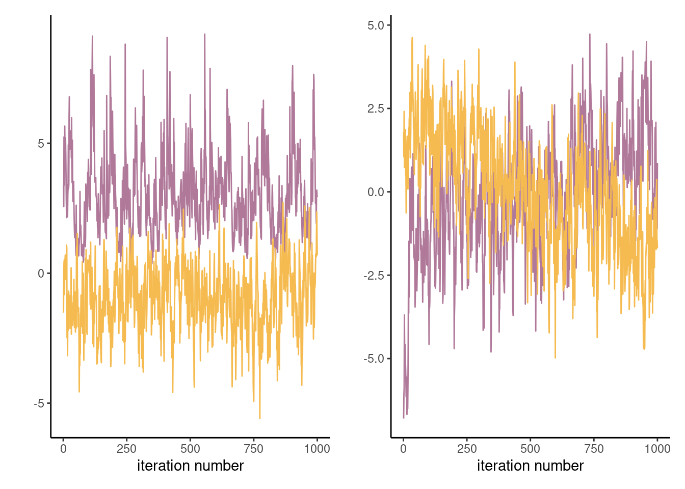
Proposition 7.1 (Gelman–Rubin diagnostic) The Gelman–Rubin diagnostic \(\widehat{R},\) introduced in Gelman and Rubin (1992) and also called potential scale reduction statistic, is obtained by considering the difference between within-chains and between-chains variance. Suppose we run \(M\) chains for \(B\) iterations, post burn in. Denoting by \(\theta_{bm}\) the \(b\)th draw of the \(m\)th chain, we compute the global average \(\overline{\theta} = B^{-1}M^{-1}\sum_{b=1}^B \sum_{m=1}^m \theta_{bm}\) and similarly the chain sample average and variances, respectively \(\overline{\theta}_m\) and \(\widehat{\sigma}^2_m\) (\(m=1, \ldots, M\)). The between-chain variance and within-chain variance estimator are \[\begin{align*} \mathsf{Va}_{\text{between}} &= \frac{B}{M-1}\sum_{m=1}^M (\overline{\theta}_m - \overline{\theta})^2\\ \mathsf{Va}_{\text{within}} &= \frac{1}{M}\sum_{m=1}^M \widehat{\sigma}^2_m \end{align*}\] and we can compute \[\begin{align*} \widehat{R} = \left(\frac{\mathsf{Va}_{\text{within}}(B-1) + \mathsf{Va}_{\text{between}}}{B\mathsf{Va}_{\text{within}}}\right)^{1/2} \end{align*}\] The potential scale reduction statistic must be, by construction, larger than 1 in large sample. Any value larger than this is indicative of problems of convergence. While the Gelman–Rubin diagnostic is frequently reported, and any value larger than 1 deemed problematic, it is not enough to have approximately \(\widehat{R}=1\) to guarantee convergence, but large values are usually indication of something being amiss. Figure 7.4 shows two instances where the chains are visually very far from having the same average and this is reflected by the large values of \(\widehat{R}.\)
Generally, it is preferable to run a single chain for a longer period than run multiple chains sequentially, as there is a cost to initializing multiple times with different starting values since we must discard initial draws. With parallel computations, multiple chains are more frequent nowadays.
7.1.1 Posterior predictive checks
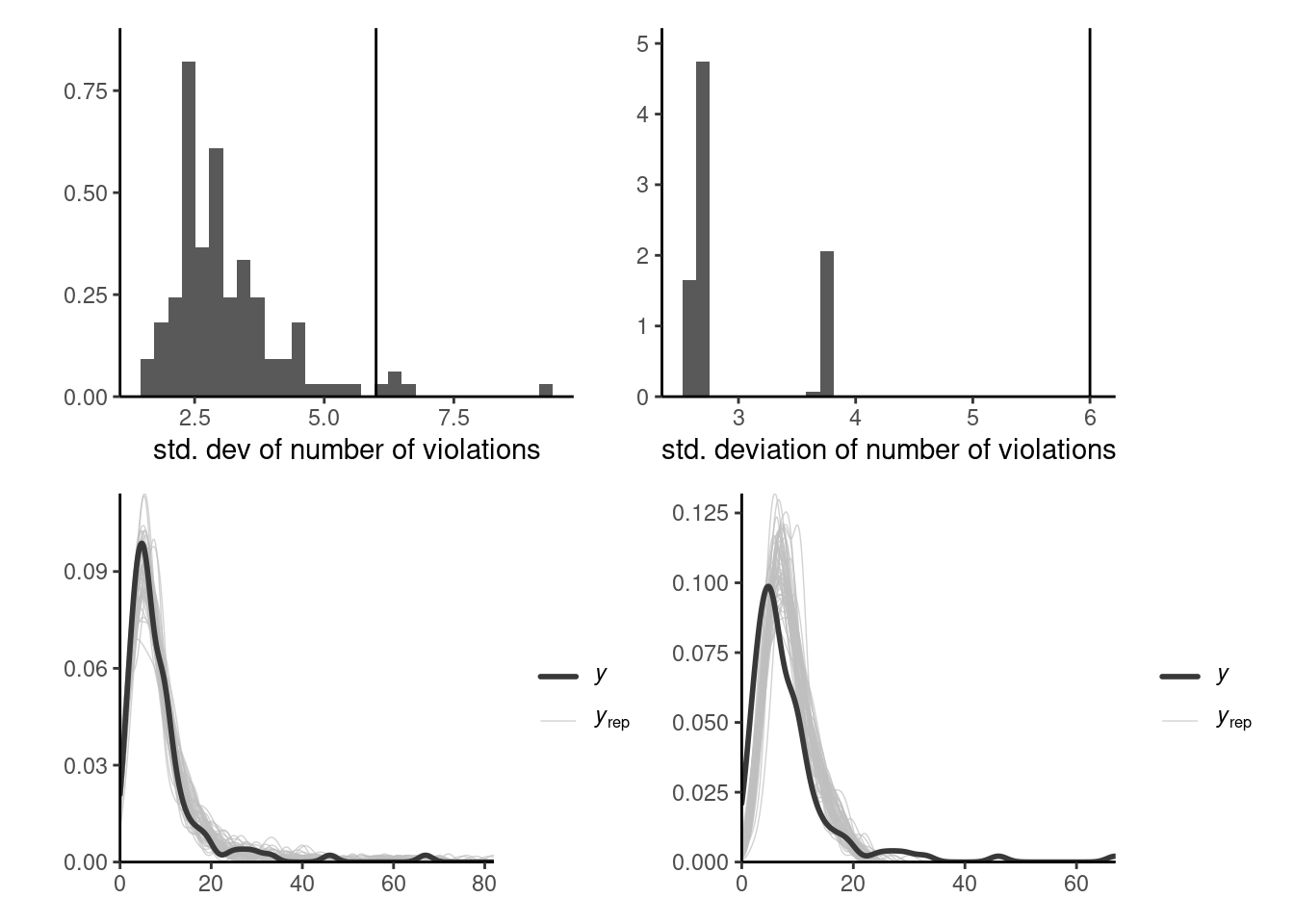
Posterior predictive checks can be used to compare models of varying complexity. One of the visual diagnostics, outlined in Gabry et al. (2019), consists in computing a summary statistic of interest from the posterior predictive (whether mean, median, quantile, skewness, etc.) which is relevant for the problem at hand and which we hope our model can adequately capture. These should be salient features of the data, and may reveal inadequate likelihood or prior information.
Suppose we have \(B\) draws from the posterior and simulate for each \(n\) observations from the posterior predictive \(p(\widetilde{\boldsymbol{y}} \mid \boldsymbol{y})\): we can benchmark summary statistics from our original data \(\boldsymbol{y}\) with the posterior predictive copies \(\widetilde{\boldsymbol{y}}_b.\) Figure 7.5 shows this for the two competing models and highlight the fact that the simpler model is not dispersed enough. Even the more complex model struggles to capture this additional heterogeneity with the additional variables. One could go back to the drawing board and consider a negative binomial model.
7.2 Information criteria
The widely applicable information criterion (Watanabe 2010) is a measure of predictive performance that approximates the cross-validation loss. Consider first the log pointwise predictive density, defined as the expected value over the posterior distribution \(p(\boldsymbol{\theta} \mid \boldsymbol{y}),\) \[\begin{align*} \mathsf{LPPD}_i = \mathsf{E}_{\boldsymbol{\theta} \mid \boldsymbol{y}} \left\{ \log p(y_i \mid \boldsymbol{\theta})\right\}. \end{align*}\] The higher the value of the predictive density \(\mathsf{LPPD}_i,\) the better the fit for that observation.
As in general information criteria, we sum over all observations, adding a penalization factor that approximates the effective number of parameters in the model, with \[\begin{align*} n\mathsf{WAIC} = -\sum_{i=1}^n \mathsf{LPPD}_i + \sum_{i=1}^n \mathsf{Va}_{\boldsymbol{\theta} \mid \boldsymbol{y}}\{\log p(y_i \mid \boldsymbol{\theta})\} \end{align*}\] where we use again the empirical variance to compute the rightmost term. When comparing competing models, we can rely on their values of \(\mathsf{WAIC}\) to discriminate about the predictive performance. To compute \(\mathsf{WAIC},\) we need to store the values of the log density of each observation, or at least minimally compute the running mean and variance accurately pointwise at storage cost \(\mathrm{O}(n).\) Note that Section 7.2 of Gelman et al. (2013) define the widely applicable information criterion as \(2n \times \mathsf{WAIC}\) to make on par with other information criteria, which are defined typically on the deviance scale and so that lower values correspond to higher predictive performance.
An older criterion which has somewhat fallen out of fashion is the deviance information criterion of Spiegelhalter et al. (2002). It is defined as \[\begin{align*} \mathsf{DIC} = -2 \ell(\widetilde{\boldsymbol{\theta}}) + 2 p_D \end{align*}\] where \(p_D\) is the posterior expectation of the deviance relative to the point estimator of the parameter \(\widetilde{\boldsymbol{\theta}}\) (e.g., the maximum a posteriori or the posterior mean) \[\begin{align*} p_D = \mathsf{E}\{D(\boldsymbol{\theta}, \widetilde{\boldsymbol{\theta}}) \mid \boldsymbol{y}\}= \int 2 \{ \ell(\widetilde{\boldsymbol{\theta}}) - \ell(\boldsymbol{\theta})\} f(\boldsymbol{\theta} \mid \boldsymbol{y}) \mathrm{d} \boldsymbol{\theta} \end{align*}\] The DIC can be easily evaluated by keeping track of the log likelihood evaluated at each posterior draw from a Markov chain Monte Carlo algorithm. The penalty term \(p_D\) is however not invariant to reparametrizations. Assuming we can derive a multivariate Gaussian approximation to the MLE under suitable regularity conditions, the \(\mathsf{DIC}\) is equivalent in large samples to \(\mathsf{AIC}.\) The \(\mathsf{DIC}\) is considered by many authors as not being a Bayesian procedure; see Spiegelhalter et al. (2014) and the discussion therein.
Criteria such as \(\mathsf{LPPD}\) and therefore \(\mathsf{WAIC}\) require some form of exchangeability, and don’t apply to cases where leave-one-out cross validation isn’t adequate, for example in spatio-temporal models.
Example 7.4 (Information criteria for smartwatch and Bayesian LASSO) For the smartwatch model, we get a value of 3.07 for the complex model and 4.5: this suggests an improvement in using individual-specific effects.
Code
# posterior: B x K matrix of posterior draws for the K coefficients
data(smartwatch, package = "hecbayes")
data(posterior_smartwatch, package = "hecbayes")
# Match coefficients to column of posterior
coef_beta <- paste0("beta[",as.integer(smartwatch$task),"]")
id_beta <- match(coef_beta, colnames(posterior_smartwatch))
coef_alpha <- paste0("alpha[",as.integer(smartwatch$id),"]")
id_alpha <- match(coef_alpha, colnames(posterior_smartwatch))
# Create containers for pointwise log likelihood and posterior predictive
B <- nrow(posterior_smartwatch)
y <- smartwatch$nviolation
n <- length(y)
loglik_pt <- matrix(nrow = B, ncol = n)
postpred <- matrix(nrow = B, ncol = n)
# Sample from posterior predictive / evaluate log likelihood
for(b in seq_len(B)){
loglik_pt[b,] <- dpois(
x = smartwatch$nviolation,
lambda = exp(posterior_smartwatch[b,id_alpha] + posterior_smartwatch[b,id_beta]),
log = TRUE)
postpred[b,] <- rpois(
n = n,
lambda = exp(posterior_smartwatch[b,id_alpha] + posterior_smartwatch[b,id_beta]))
}
# Watanabe's widely available information criterion
WAIC <- function(loglik_pt){
-mean(apply(loglik_pt, 2, mean)) + mean(apply(loglik_pt, 2, var))
}
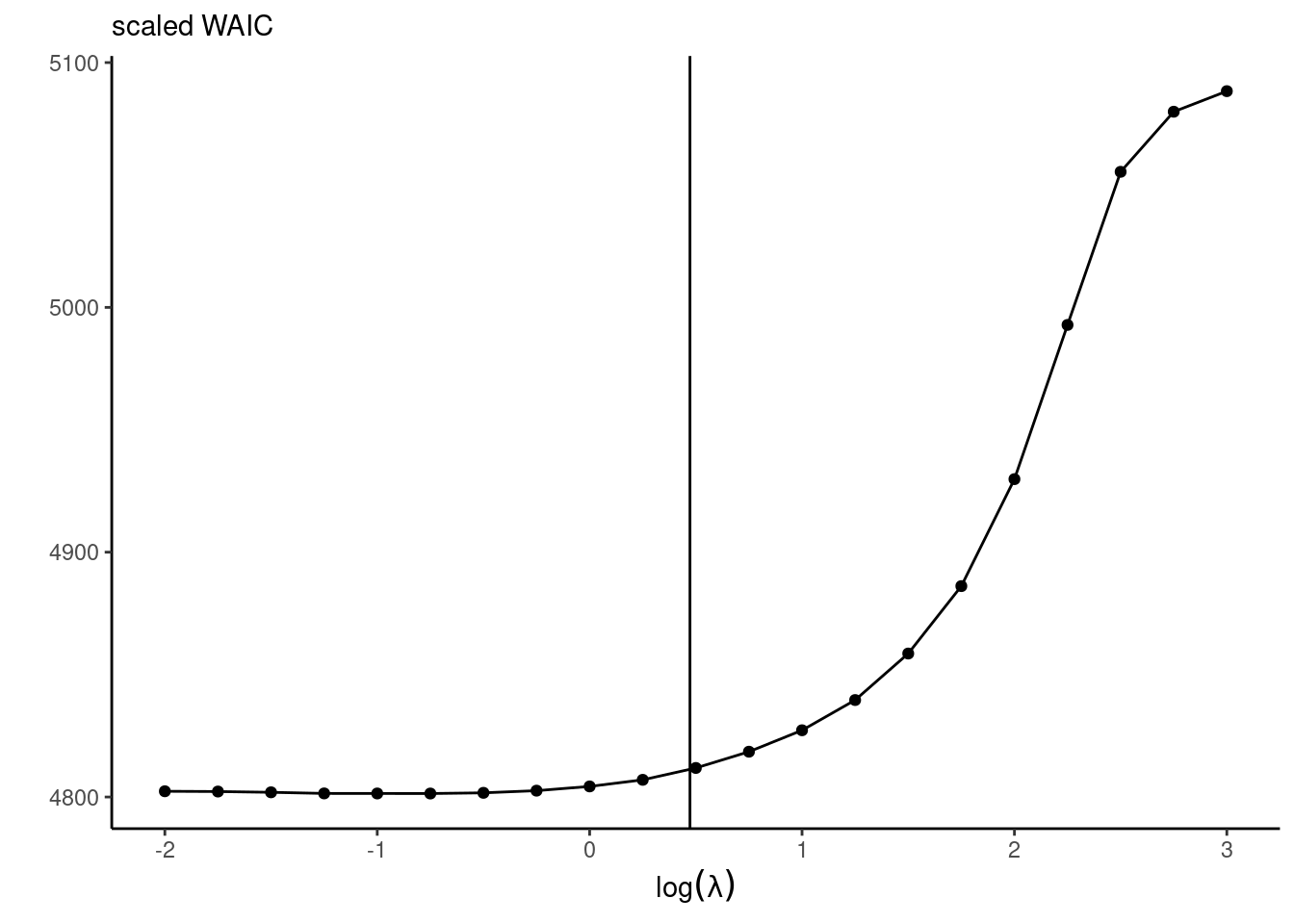
WAIC(loglik_pt)We can also look at the predictive performance. For the diabetes data application with the Bayesian LASSO with fixed \(\lambda,\) the predictive performance is a trade-off between the effective number of parameter (with larger penalties translating into smaller number of parameters) and the goodness-of-fit. Figure 7.6 shows that the decrease in predictive performance is severe when estimates are shrunk towards 0, but the model performs equally well for small penalties.
Ideally, one would measure the predictive performance using the leave-one-out predictive distribution for observation \(i\) given all the rest, \(p(y_i \mid \boldsymbol{y}_{-i}),\) to avoid double dipping — the latter is computationally intensive to obtain because it would require running \(n\) Markov chains with \(n-1\) observations each, but we can get a good approximation using importance sampling, as proposed in eq. 25 of Section 7 of Gelfand and Dey (1994).
Proposition 7.2 (Marginal predictive check) To check the goodness-of-fit, we turn to the posterior predictive distribution. For each posterior draw and each observation, we generate a sample from the posterior predictive, resulting in an \(n \times B\) matrix. We can then for each observation \(y_i\) compare the latter with the simulated samples \(y_{i,b}^{\mathrm{rep}}\) for posterior sample \(\boldsymbol{\theta}_b.\) We compute \(\Pr(y_i \geq y_{i}^{\mathrm{rep}})\) by Monte Carlo, by looking at the sample proportion that are more extreme. Values close to zero or one may indicate outliers.
To avoid double dipping, we can check model adequacy by comparing the leave-one-cross validation predictive draws with the observation.
Proposition 7.3 (Cross-validation predictive density) Consider estimation of the leave-one predictive density under the hypothesis that the likelihood factorizes as \(L(\boldsymbol{\theta}; \boldsymbol{y}) = \prod_{i=1}^n f_i(y_i; \boldsymbol{\theta});\) where \(f_i\) is the density or mass function of the \(i\)th observation. Then, with weights \[\begin{align*}
w_i(\boldsymbol{\theta}) = \frac{p(\boldsymbol{\theta} \mid \boldsymbol{y}_{-i})}{p(\boldsymbol{\theta} \mid \boldsymbol{y})} \stackrel{\boldsymbol{\theta}}{\propto} \frac{1}{f_i(y_i; \boldsymbol{\theta})}
\end{align*}\] we can write the leave-one-out posterior predictive as \[\begin{align*}
p(y_i \mid \boldsymbol{y}_{-i}) &= \int_{\boldsymbol{\Theta}} f_i(y_i; \boldsymbol{\theta}) p(\boldsymbol{\theta} \mid \boldsymbol{y}_{-i}) \mathrm{d} \boldsymbol{\theta}
\\& = \int_{\boldsymbol{\Theta}} f(y_i; \boldsymbol{\theta}) w_i(\boldsymbol{\theta}) p(\boldsymbol{\theta} \mid \boldsymbol{y}) \mathrm{d} \boldsymbol{\theta}.
\end{align*}\] This formula suggests the importance sampling estimator (cf. Proposition 4.4) for a sample of size \(B\) from the posterior \(p(\boldsymbol{\theta} \mid \boldsymbol{y})\) \[\begin{align*}
\widehat{p}(y_i \mid \boldsymbol{y}_{-i}) = \frac{\sum_{b=1}^B f_i(y_i; \boldsymbol{\theta}_b) w_i(\boldsymbol{\theta}_b)}{\sum_{b=1}^Bw_i(\boldsymbol{\theta}_b)} = B \left\{\sum_{b=1}^B \frac{1}{f_i (y_i; \boldsymbol{\theta}_b)}\right\}^{-1}.
\end{align*}\] This estimator takes the form of an harmonic mean, which can have very large variance due to some weights dominating the fit. Vehtari, Gelman, and Gabry (2017) proposed using Pareto smoothed importance sampling (Vehtari et al. 2024) to avoid overly large weights; this method is implemented in the loo R package.
Suppose we have matrices of size \(n \times B\) containing the posterior predictive draws \(y_{i,b}^{\mathrm{rep}}\) associated with each posterior vector \(\boldsymbol{\theta}_b\) and the weights \(w_{i,b} = 1/f_i (y_i \mid \boldsymbol{\theta}_b)\) from the importance sampling estimator. We can then compute the probability integral transform with importance sampling \[\begin{align*} \widehat{p}_i^{\mathrm{loo}} = \Pr(y_i^{\mathrm{rep}} \leq y_i \mid \boldsymbol{y}_{-i}) \approx \frac{\sum_{b=1}^B \mathrm{I}(y_i^{\mathrm{rep}} \leq y_i)w_{i,b}}{\sum_{b=1}^B w_{i,b}}, \qquad i =1,\ldots, n \end{align*}\] We can then create a probability-probability plot with these values by comparing the \(n\) with ordered quantiles with uniform plotting positions. The values \(\widehat{p}_i^{\mathrm{loo}}\) should be approximately uniform if the model was perfectly calibrated. Figure 7.7 shows two examples of these.
Code
is_wgt <- exp(-loglik_pt) # log weights
# importance sampling estimator
ploo <- numeric(n)
for(i in seq_along(y)){
 ploo[i] <- weighted.mean(x = I(postpred[,i] <= y[i]), w = is_wgt[,i])
}
ggplot(data = data.frame(ploo = sort(ploo), punif = ppoints(n)),
       mapping = aes(x = punif, y = ploo)) +
  geom_abline(slope = 1, intercept = 0) +
  geom_point() +
  labs(x = "uniform", y = "LOO-PIT")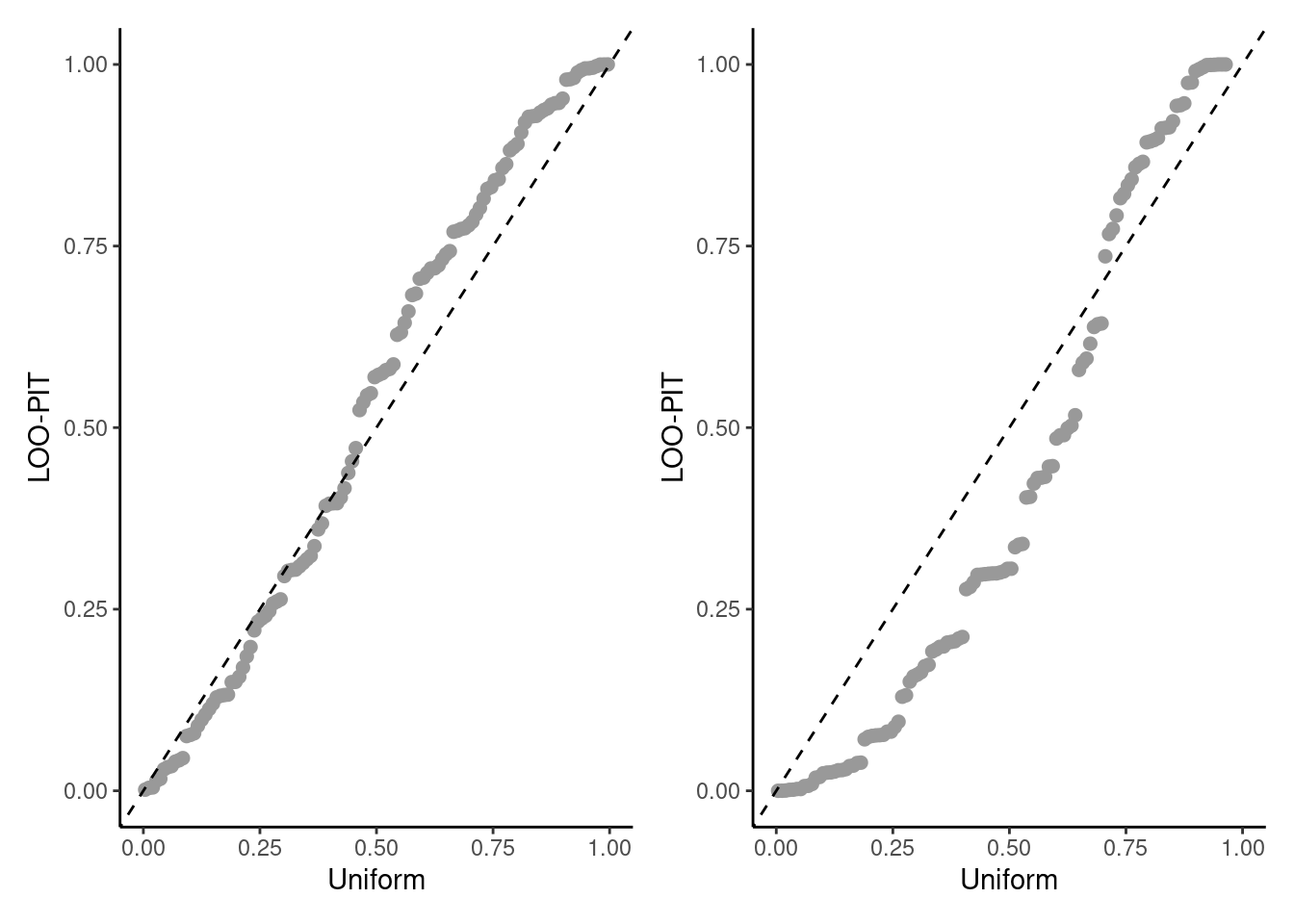
7.3 Computational strategies
The data augmentation strategies considered in Section 6.1 helps to simplify the likelihood and thereby reduce the cost of each iteration. However, latent variables are imputed conditional on current parameter values \(\boldsymbol{\theta}_a\): the higher the number of variables, the more the model will concentrate around current values of \(\boldsymbol{\theta}_a\), which leads to slow mixing.
There are two main strategies to deal with this problem: blocking the random effects together and simulating them jointly to improve mixing, and marginalizing out over some of the latent variables.
Example 7.5 (Marginalization in Gaussian models) To illustrate this fact, consider a hierarchical Gaussian model of the form \[\begin{align*} \boldsymbol{Y} = \mathbf{X}\boldsymbol{\beta} + \mathbf{Z}\boldsymbol{B} + \boldsymbol{\varepsilon} \end{align*}\] where \(\mathbf{X}\) is an \(n \times p\) design matrix with centered inputs, \(\boldsymbol{\beta} \sim \mathsf{Gauss}(\boldsymbol{0}_p, \sigma^2\mathbf{I}_p),\) \(\boldsymbol{B}\sim \mathsf{Gauss}_q(\boldsymbol{0}_q, \boldsymbol{\Omega})\) are random effects and \(\boldsymbol{\varepsilon} \sim \mathsf{Gauss}_n(\boldsymbol{0}_n, \kappa^2\mathbf{I}_n)\) are independent white noise.
We can write \[\begin{align*} \boldsymbol{Y} \mid \mathbf{\beta}, \boldsymbol{B} &\sim \mathsf{Gauss}_n(\mathbf{X}\boldsymbol{\beta} + \mathbf{Z}\boldsymbol{B}, \sigma^2\mathbf{I}_p)\\ \boldsymbol{Y} \mid \mathbf{\beta} &\sim \mathsf{Gauss}_n(\mathbf{X}\boldsymbol{\beta}, \mathbf{Q}^{-1}), \end{align*}\] where the second line corresponds to marginalizing out the random effects \(\boldsymbol{B}.\) This reduces the number of parameters to draw, but the likelihood evaluation is more costly due to \(\mathbf{Q}^{-1}\). If, as is often the case, \(\boldsymbol{\Omega}^{-1}\) and \(\mathbf{Z}\) are sparse matrices, the full precision matrix can be efficiently computed using Shermann–Morisson–Woodbury identity as \[\begin{align*} \mathbf{Q}^{-1} &= \mathbf{Z}\boldsymbol{\Omega}^{-1}\mathbf{Z}^\top + \kappa^2 \mathbf{I}_n,\\ \kappa^2\mathbf{Q} & = \mathbf{I}_n - \mathbf{Z} \boldsymbol{G}^{-1} \mathbf{Z}^\top,\\ \boldsymbol{G} &= \mathbf{Z}^\top\mathbf{Z} + \kappa^2 \boldsymbol{\Omega}^{-1} \end{align*}\] Section 3.1 of Nychka et al. (2015) details efficient ways of calculating the quadratic form involving \(\mathbf{Q}\) and it’s determinant.
Proposition 7.4 (Pseudo marginal) Another option proposed by Andrieu and Roberts (2009) based on an original idea from Beaumont (2003) relies on pseudo marginalization, where integration is done via Monte Carlo sampling. Specifically, suppose that we are ultimately interested in \[p(\boldsymbol{\theta})= \int p(\boldsymbol{\theta}, \boldsymbol{z}) \mathrm{d} \boldsymbol{z},\] but that for this purpose we normally sample from both parameters. Given a proposal \(\boldsymbol{\theta}\) and \(q_1(\boldsymbol{\theta})\) and subsequently \(L\) draws once from \(q_2(\boldsymbol{z} \mid \boldsymbol{\theta})\) for the nuisance, we can approximate the marginal using, e.g., importance sampling as \[\begin{align*} \widehat{p}(\boldsymbol{\theta}; \boldsymbol{z}) = \frac{1}{L} \sum_{l=1}^L \frac{p(\boldsymbol{\theta}, \boldsymbol{z}_l)}{q_2(\boldsymbol{z}_l, \boldsymbol{\theta})}. \end{align*}\] We then run a Markov chain on an augmented state space \(\boldsymbol{\Theta} \times \mathcal{Z}^L\), with Metropolis–Hastings acceptance ratio of \[\begin{align*} \frac{\widehat{p}(\boldsymbol{\theta}^{\star}; \boldsymbol{z}_{1,t}^{\star}, \boldsymbol{z}_{L,t}^{\star})}{ \widehat{p}(\boldsymbol{\theta}_t; \boldsymbol{z}_{1,t-1}, \ldots, \boldsymbol{z}_{L, t-1})}\frac{q_1(\boldsymbol{\theta}_{t-1} \mid \boldsymbol{\theta}^{\star}_t)}{q_1(\boldsymbol{\theta}^{\star}_t \mid \boldsymbol{\theta}_{t-1})}. \end{align*}\] Note that the terms involving \(\prod_{l=1}^L q_2(\boldsymbol{z}_{l}; \boldsymbol{\theta})\) do not appear because they cancel out, as they are also part of the augmented state space likelihood.
The remarkable feature of the pseudo marginal approach is that even if our average approximation \(\widehat{p}\) to the marginal is noisy, the marginal posterior of this Markov chain is the same as the original target.
Compared to regular data augmentation, we must store the full vector \(\boldsymbol{z}^{\star}_1, \ldots, \boldsymbol{z}^{\star}_L\) and perform \(L\) evaluations of the augmented likelihood. The values of \(\boldsymbol{z}\), if accepted, are stored for the next evaluation of the ratio.
The idea of pseudo-marginal extends beyond the user case presented above, as as long as we have an unbiased non-negative estimator of the likelihood \(\mathsf{E}\{\widehat{p}(\boldsymbol{\theta})\}=p(\boldsymbol{\theta})\), even when the likelihood itself is intractable. This is useful for models where we can approximate the likelihood by simulation, like for particle filters. Pseudo marginal MCMC algorithms are notorious for yielding sticky chains.
Proposition 7.5 (Blocking) When parameters of the vector \(\boldsymbol{\theta}\) that we wish to sample are strongly correlated, it is advisable when possible to simulate them jointly. Because the unnormalized posterior is evaluated at each step conditional on all values, the Markov chain will be making incremental moves and mix slowly if we sample them one step at a time.
Before showcasing the effect of blocking and joint updates, we present another example of data augmentation using Example 6.2.
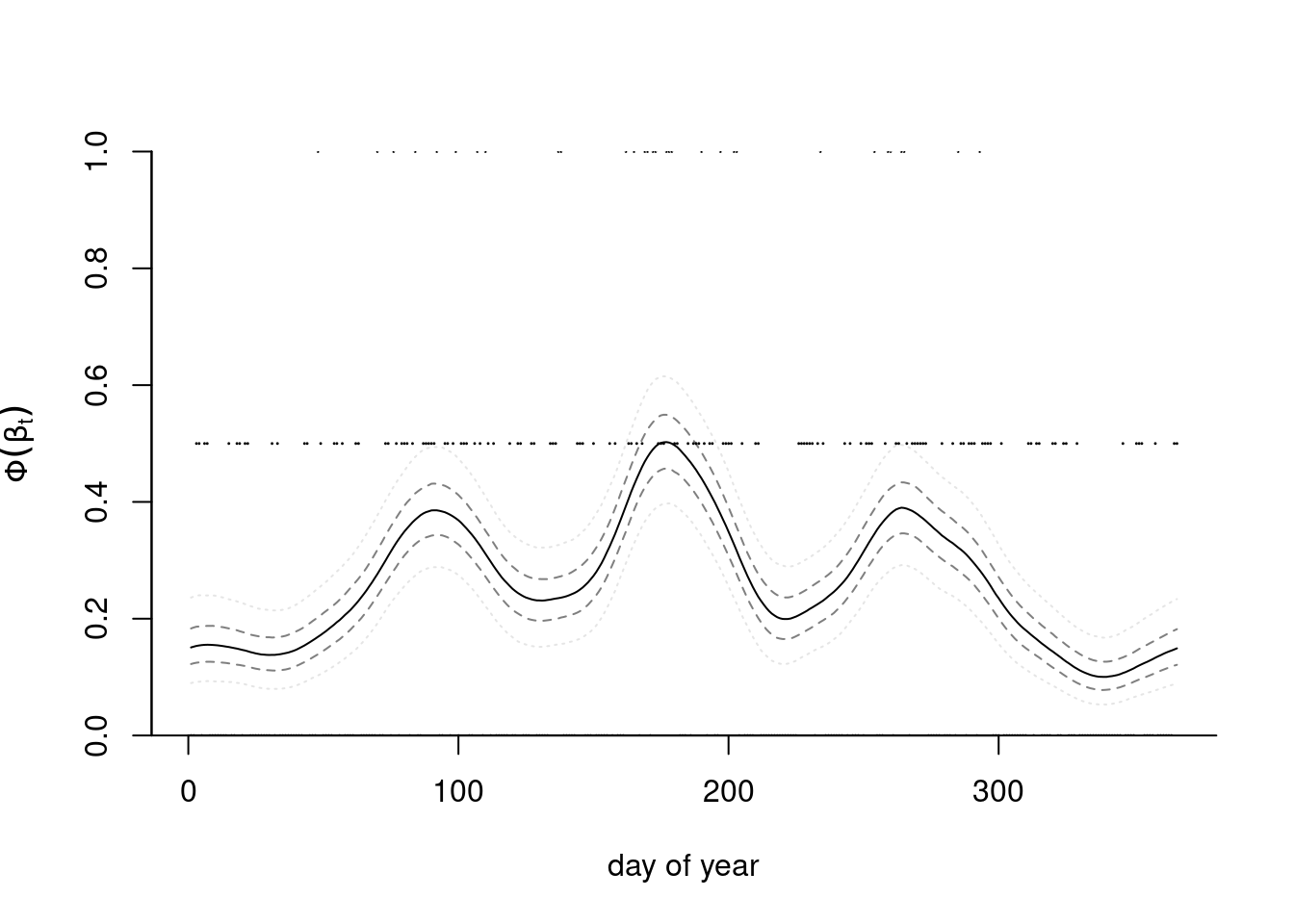
Example 7.6 (Tokyo rainfall) We consider data from Kitagawa (1987) that provide a binomial time series giving the number of days in years 1983 and 1984 (a leap year) in which there was more than 1mm of rain in Tokyo. These data and the model we consider are discussed in in section 4.3.4 of Rue and Held (2005). We thus have \(T=366\) days and \(n_t \in \{1,2\}\) \((t=1, \ldots, T)\) the number of observations in day \(t\) and \(y_t=\{0,\ldots, n_t\}\) the number of days with rain. The objective is to obtain a smoothed probability of rain. The underlying probit model considered takes \(Y_t \mid n_t, p_t \sim \mathsf{binom}(n_t, p_t)\) and \(p_t = \Phi(\beta_t).\)
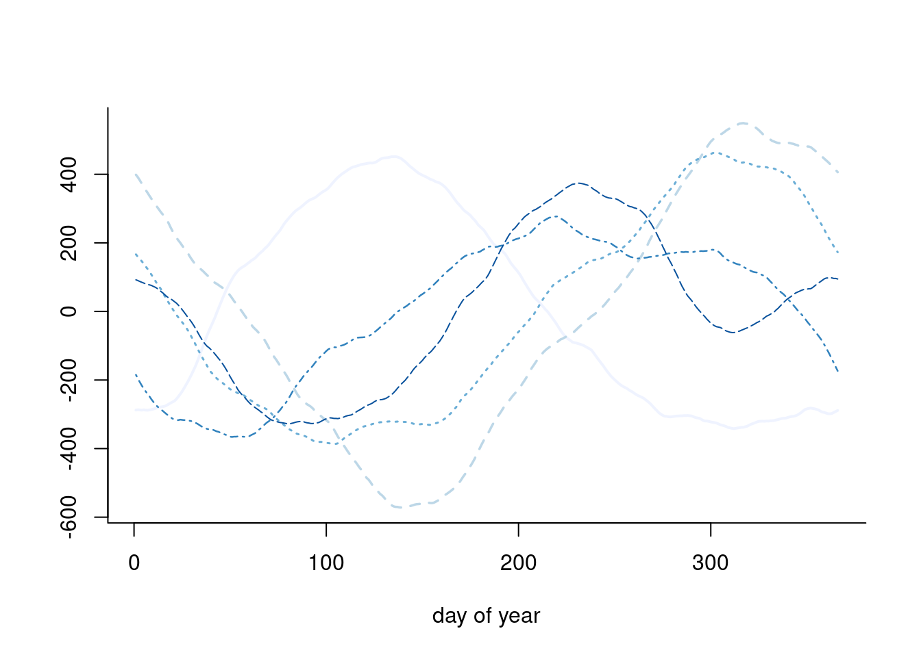
We specify the random effects \(\boldsymbol{\beta} \sim \mathsf{Gauss}_{T}(\boldsymbol{0}, \tau^{-1}\mathbf{Q}^{-1}),\) where \(\mathbf{Q}\) is a \(T \times T\) precision matrix that encodes the local dependence. A circular random walk structure of order 2 is used to model the smooth curves by smoothing over neighbors, and enforces small second derivative. This is a suitable prior because it enforces no constraint on the mean structure. This amounts to specifying the process with \[\begin{align*} \Delta^2\beta_t &= (\beta_{t+1} - \beta_t) - (\beta_t - \beta_{t-1}) \\&=-\beta_{t-1} +2 \beta_t - \beta_{t+1} \sim \mathsf{Gauss}(0, \tau^{-1}), \qquad t \in \mathbb{N} \mod 366. \end{align*}\] This yields an intrinsic Gaussian Markov random field with a circulant precision matrix \(\tau\mathbf{Q}=\tau\mathbf{GG^\top}\) of rank \(T-1,\) where \[\begin{align*} \mathbf{G} &= \begin{pmatrix} 2 & -1 & 0 & 0 & \cdots & -1\\ -1 & 2 & -1 & 0 & \ddots & 0 \\ 0 & -1 & 2 & -1 & \ddots & 0 \\ \vdots & \ddots & \ddots & \ddots & \ddots & \vdots \\ -1 & 0 & 0 & 0 & \cdots & 2 \end{pmatrix}, \\ \mathbf{Q} &= \begin{pmatrix} 6 & -4 & 1 & 0 & \cdots & 1 & -4\\ -4 & 6 & -4 & 1 & \ddots & 0 & 1 \\ 1 & -4 & 6 & -4 & \ddots & 0 & 0 \\ \vdots & \ddots & \ddots & \ddots & \ddots & \ddots & \vdots \\ -4 & 1 & 0 & 0 & \cdots & -4 & 6 \end{pmatrix}. \end{align*}\] Because of the linear dependency, the determinant of \(\mathbf{Q}\) is zero. The contribution from the latent mean parameters is multivariate Gaussian and we exploit for computations the sparsity of the precision matrix \(\mathbf{Q}.\) Figure 7.8 shows five draws from the prior model, which loops back between December 31st and January 1st, and is rather smooth.
We can perform data augmentation by imputing Gaussian variables, say \(\{z_{t,i}\}\) following Example 6.2 from truncated Gaussian, where \(z_{t,i} = \beta_t + \varepsilon_{t,i}\) and \(\varepsilon_{t,i} \sim \mathsf{Gauss}(0,1)\) are independent standard Gaussian and \[\begin{align*} z_{t,i} \mid y_{t,i}, \beta_t \sim \begin{cases} \mathsf{trunc. Gauss}(\beta_t, 1, -\infty, 0) & y_{t,i} = 0 \\ \mathsf{trunc. Gauss}(\beta_t, 1, 0, \infty) & y_{t,i} =1 \end{cases} \end{align*}\] The posterior is proportional to \[\begin{align*} p(\boldsymbol{\beta} \mid \tau)p(\tau)\prod_{t=1}^{T}\prod_{i=1}^{n_t}p(y_{t,i} \mid z_{t,i}) p(z_{t,i} \mid \beta_t) \end{align*}\] and once we have imputed the Gaussian latent vectors, we can work directly with the values of \(z_t = \sum_{i=1}^{n_t} z_{i,t}.\) The posterior then becomes \[\begin{align*} p(\boldsymbol{\beta}, \tau) &\propto \tau^{(n-1)/2}\exp \left( - \frac{\tau}{2} \boldsymbol{\beta}^\top \mathbf{Q} \boldsymbol{\beta}\right)\tau^{a-1}\exp(-\tau b)\\& \quad \times \exp\left\{ - \frac{1}{2} (\boldsymbol{z}/\boldsymbol{n} - \boldsymbol{\beta})^\top \mathrm{diag}(\boldsymbol{n})(\boldsymbol{z}/\boldsymbol{n} - \boldsymbol{\beta})\right\} \end{align*}\] where \(\boldsymbol{z} = (z_1, \ldots, z_T).\) Completing the quadratic form shows that \[\begin{align*} \boldsymbol{\beta} \mid \boldsymbol{z}, \tau &\sim \mathsf{Gauss}_T\left[\left\{\tau \mathbf{Q} + \mathrm{diag}(\boldsymbol{n})\right\}^{-1} \boldsymbol{z}, \left\{\tau \mathbf{Q} + \mathrm{diag}(\boldsymbol{n})\right\}^{-1}\right]\\ \tau \mid \boldsymbol{\beta} & \sim \mathsf{gamma}\left( \frac{n-1}{2} + a, \frac{\boldsymbol{\beta}^\top \mathbf{Q}\boldsymbol{\beta}}{2} + b \right) \end{align*}\]
library(Matrix)
library(TruncatedNormal)
data(tokyorain, package = "hecbayes")
# Aggregate data
tokyo <- tokyorain |>
   dplyr::group_by(day) |>
   dplyr::summarize(y = sum(y), n = dplyr::n())
nt <- 366L
# Circulant random walk of order two precision matrix
Q <- hecbayes::crw_Q(d = nt, type = "rw2", sparse = TRUE)
# Sparse Cholesky root
cholQ <- Matrix::chol(Q)
N <- Matrix::Diagonal(n = nt, x = tokyo$n)
# Create containers
B <- 1e4L # number of draws
beta_s <- matrix(nrow = B, ncol = nt)
x_s <- matrix(nrow = B, ncol = nt)
tau_s <- numeric(B)
# Initial values
beta <- rep(0, nt)
tau <- 1000
# Hyperprior parameter values
tau_a <- 1
tau_b <- 0.0001
# Gibbs sampling
for(b in seq_len(B)){
  # Step 1: data augmentation
  x <- TruncatedNormal::rtnorm(
    n = 1,  mu = beta[tokyorain$day], sd = 1,
    lb = ifelse(tokyorain$y == 0, -Inf, 0),
    ub = ifelse(tokyorain$y == 0, 0, Inf))
  tx <- aggregate(x = x, by = list(tokyorain$day), FUN = sum)$x
  x_s[b,] <- tx
  # Step 2: Simulate random effects in block
  beta <- beta_s[b,] <- c(hecbayes::rGaussQ(
    n = 1,
    b = tx,
    Q = tau * Q + N))
# Simulate precision
  tau <- tau_s[b] <- rgamma(
    n = 1,
    shape = (nt-1)/2 + tau_a,
    rate = 0.5*as.numeric(crossprod(cholQ %*% beta)) + tau_b)
  # if beta is VERY smooth, then precision is large
}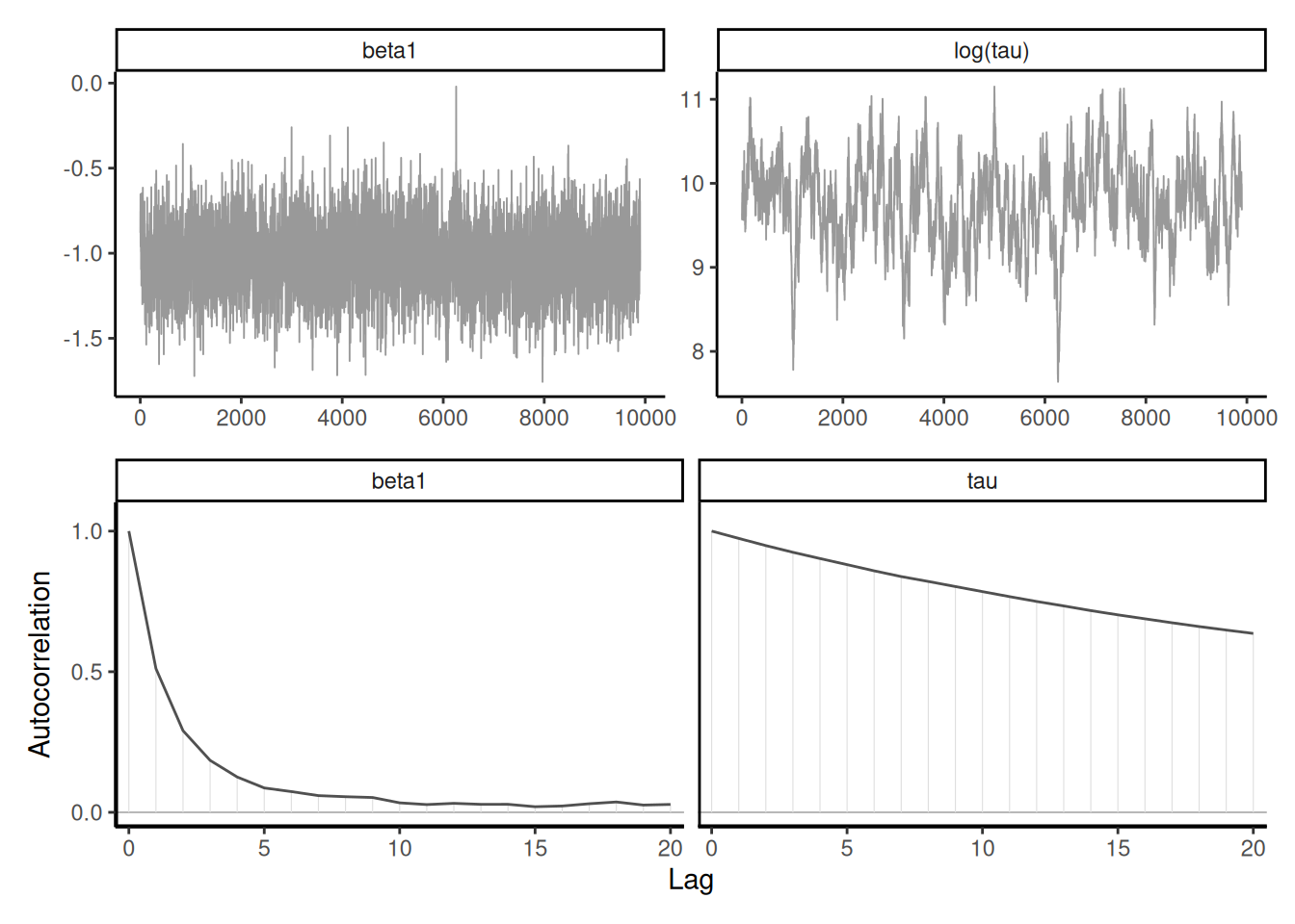
Example 7.7 (Blocking) We revisit Example 7.6 with two modifications: imputing one parameter \(\beta_t\) at a time using random scan Gibbs step, which leads to slower mixing but univariate updates, and a joint update that first draws \(\tau^{\star}\) from some proposal distribution, then sample conditional on that value generates the \(\boldsymbol{\beta}\) vector and proposes acceptance using a Metropolis step.
A different (less efficient) strategy would be to simulate the \(\beta_t\) terms one at a time using a random scan Gibbs, i.e., picking \(t_0 \in \{1, \ldots, 366\}\) and looping over indices. This yields higher autocorrelation between components than sampling by block.
  # Compute mean vector for betas
  mbeta <- Matrix::solve(a = tau*Q + N, b = tx)
  # weights of precision for neighbours
  nw <- c(1, -4, -4, 1)
  # Sample an index at random
  st <- sample.int(nt, 1)
  for(i in (st + seq_len(nt)) %% nt + 1L){
   # Indices of the non-zero entries for row Q[i,]
  nh <- c(i-3, i-2, i, i+1) %% 366 + 1
  prec <- tau * 6 + tokyo$n[i]
  condmean <- mbeta[i] - sum(nw*(beta[nh] - mbeta[nh])) * tau / prec
    beta[i] <- rnorm(n = 1, mean = condmean, sd = 1/sqrt(prec))
  }
  beta_s[b,] <- beta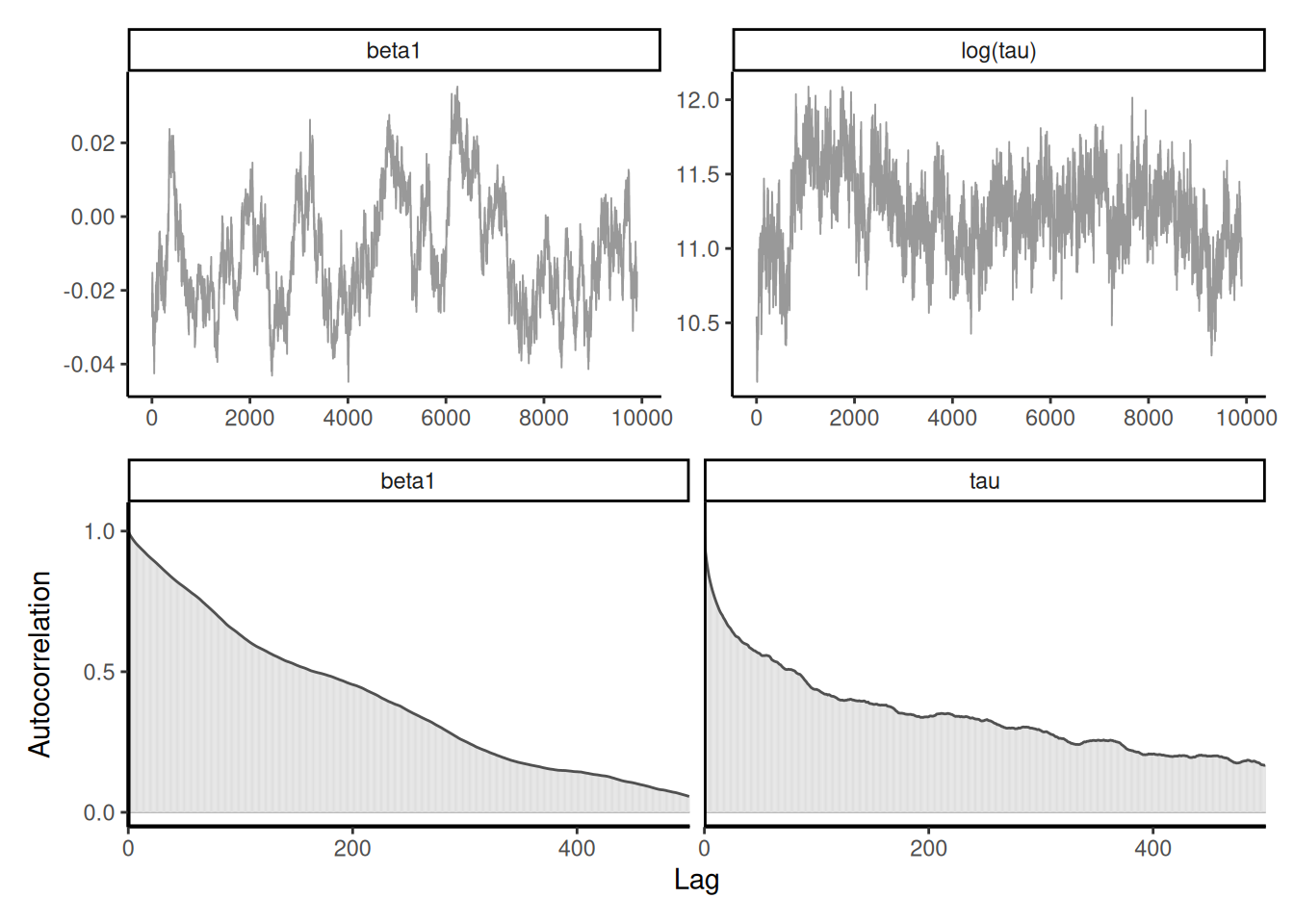
Instead of making things worst, we can try to improve upon our initial sampler by simulating first a proposal \(\tau^{\star}\) using a random walk Metropolis (on the log scale) or some other proposal \(q(\tau^{\star}; \tau),\) then drawing from the full conditional \(\boldsymbol{\beta} \mid \boldsymbol{z}, \tau^{\star}\) and accepting/rejecting the whole move. In doing this, all terms that depend on \(\boldsymbol{\beta}\) cancel out, and the term \(p(\tau^{\star}, \boldsymbol{\beta}^{\star} \mid \tau)/\{q(\tau^{\star}; \tau)p(\boldsymbol{\beta}^{\star} \mid \tau^{\star})\}\) in the acceptance ratio becomes \[\begin{align*} \frac{\tau_t^{\star(n-1)/2} p(\tau_t^{\star})\exp \left\{-\frac{1}{2}\boldsymbol{z}^\top(\boldsymbol{z}/\boldsymbol{n})\right\}}{q(\tau^{\star}; \tau) \left| \tau^{\star}\mathbf{Q} + \mathrm{diag}(\boldsymbol{n})\right|\exp \left[-\frac{1}{2}\boldsymbol{z}^\top \left\{\tau^{\star}\mathbf{Q} + \mathrm{diag}(\boldsymbol{n})\right\}^{-1}\boldsymbol{z}\right]} \end{align*}\]
A second alternative is to ditch altogether the data augmentation step and write the unnormalized log posterior for \(\boldsymbol{\beta}\) as \[\begin{align*} \log p(\boldsymbol{\beta} \mid \boldsymbol{y}) \stackrel{\boldsymbol{\beta}}{\propto} - \frac{\tau}{2} \boldsymbol{\beta}^\top \mathbf{Q} \boldsymbol{\beta} + \sum_{t=1}^{366} y_{t} \log \Phi(\beta_t) + (n_t-y_{t}) \log\{1-\Phi(\beta_t)\} \end{align*}\] and do a quadratic approximation to the posterior by doing a Taylor expansion of the terms \(\log p(y_{t} \mid \beta_{t})\) around the current value of the draw for \(\boldsymbol{\beta}.\) Given that observations are conditionally independent, we have a sum of independent terms \(\ell(\boldsymbol{y}; \boldsymbol{\beta}) = \sum_{t=1}^{366}\log p(y_t \mid \beta_t)\) and this yields, expanding around \(\boldsymbol{\beta}^0\), the Gaussian Markov field proposal \[\begin{align*} q(\boldsymbol{\beta} \mid \tau, \boldsymbol{\beta}^0) \sim \mathsf{Gauss}_{366}\left[\ell'(\boldsymbol{\beta}^0), \tau\mathbf{Q} + \mathrm{diag}\{\ell''(\boldsymbol{\beta}^0)\}\right]. \end{align*}\] Indeed, because of conditional independence, the \(j\)th element of \(\ell'\) and \(\ell''\) are \[\begin{align*} \ell'(\boldsymbol{\beta}^0)_j = \left. \frac{\partial \ell(y_j; \beta_j)}{\partial \beta_j}\right|_{\beta_j = \beta_j^0}, \quad \ell''(\boldsymbol{\beta}^0)_j = \left. \frac{\partial^2 \ell(y_j; \beta_j)}{\partial \beta_j^2}\right|_{\beta_j = \beta_j^0}. \end{align*}\] We can then simulate \(\tau\) using an random walk step, then propose \(\boldsymbol{\beta}\) conditional on this value using the Gaussian approximation above and accept/reject the pair \((\tau, \boldsymbol{\beta})\) using a Metropolis step. As for the Metropolis-adjusted Langevin algorithm, we need to compute the backward move for the acceptance ratio. We refer to Section 4.4.1 of Rue and Held (2005) for more details.
Strong dependence can be fixed by blocking (often via forward sampling), but perhaps conterintuitively also be adding additional redundant parameters. Gelman et al. (2013) consider a simple hierarchical random effect model in which the range of the random effects is severely constrained by the variance.
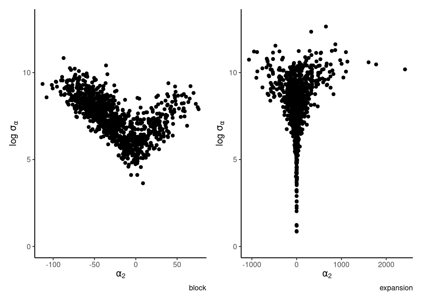
Example 7.8 (Parameter expansion) Consider a one-way ANOVA with a single observation per group, where for \(i=1, \ldots, n,\) we have \[\begin{align*} Y_{i} &\sim \mathsf{Gauss}(\mu + \alpha_i, s^2_i) \\ \alpha_i &\sim \mathsf{Gauss}(0, \sigma^2_\alpha) \end{align*}\] and an improper prior for the mean \(p(\mu) \propto 1.\) If there are \(K\) groups, then the group-specific mean is \(\mu+\alpha_k\), and there is a redundant parameter. In the Bayesian setting, the parameters are weakly identifiable because of the prior on \(\boldsymbol{\alpha}\), but the geometry is such that \(\alpha_k \to 0\) as \(\sigma^2_{\alpha} \to 0.\) See Section 5.5 on p. 119 of Gelman et al. (2013) for more details.
We can improve mixing by adding the redundant parameter \(\nu\) (Gelman et al. 2008) common to each observation \[\begin{align*} Y_{i} &\sim \mathsf{Gauss}(\mu + \nu\xi_i, s^2_i) \\ \xi_i &\sim \mathsf{Gauss}(0, \sigma^2_\xi) \end{align*}\] so that \(\alpha_j = \nu \xi_j\) and \(\sigma_\alpha = |\nu|\sigma_\xi.\) The common parameter \(\nu\) controls both the variance and the amplitude of the coefficients.
Consider the eight school data from Educational Testing Service (ETS), featured prominently in Gelman et al. (2013). The data shows results of randomized experiments in eight different schools to estimate the effect of coaching on SAT-V scores. The data consist of estimated treatment mean difference \(y_1, \ldots, y_8\) and their standard errors \(\sigma_1, \ldots, s_8\). The data size are large, so the average treatment effect (ATE) can be considered Gaussian and the school-specific standard errors \(s_j\) are treated as a known quantity.
We can devise different Gibbs sampling from this problem. The naive Gibbs sampler, which iterates between conditionals of \(p(\boldsymbol{\alpha} \mid \boldsymbol{y}, \boldsymbol{s}^2, \mu, \sigma^2_{\alpha})\) and \(p(\mu \mid \boldsymbol{y}, \boldsymbol{s}^2, \boldsymbol{\alpha})\) leads to strong autocorrelation. A better strategy is to marginalize over the global mean \(\mu\) and simulate from \(p(\boldsymbol{\alpha} \mid \boldsymbol{y}, \boldsymbol{s}^2, \sigma^2_{\alpha})\) instead. We get then the conditionals \[\begin{align*} \alpha_i \mid y_i, s_i^2, \sigma^2_{\alpha} &\sim \mathsf{Gauss}\left\{ \left(s^{-2}_i + \sigma^{-2}_{\alpha}\right)^{-1}\frac{y_i}{s^2_j}, \left(s^{-2}_i + \sigma^{-2}_{\alpha}\right)^{-1}\right\}\\ \mu \mid \boldsymbol{y}, \boldsymbol{s}^2, \boldsymbol{\alpha} & \sim \mathsf{Gauss}\left( s^2_{\mu} \sum_{j=1}^8 \frac{y_i-\alpha_i}{s^2_j}, s^2_{\mu}\right)\\ \sigma^2_{\alpha} \mid \boldsymbol{\alpha} &\sim \mathsf{inv. gamma}\left( \frac{n-1}{2}, \frac{\sum_{j=1}^8 \alpha_j^2}{2}\right) \end{align*}\] where \(s^{-2}_{\mu} =\sum_{j=1}^8 s_j^{-2}.\)
The parameter expansion sampler proceeds in exactly the same way with the same conditionals for \(\sigma_{\xi}^2\) and \(\boldsymbol{\xi}\) as above; the only additional step is \[\begin{align*} \nu \mid \boldsymbol{y}, \boldsymbol{s}^2, \boldsymbol{\xi} & \sim \mathsf{Gauss}\left\{ \left( \sum_{j=1}^8 \xi_j^2/s_j^2\right)^{-1} \sum_{j=1}^8 \xi_j(y_j-\mu)/s^2_j, \left( \sum_{j=1}^8 \xi_j^2/s_j^2\right)^{-1}\right\}. \end{align*}\] After each update, we then save the progress of \(\alpha_j = \nu \xi_j\) and \(\sigma_\alpha = |\nu|\sigma_\xi,\) as the other parameters are not identifiable on their own. The redundant parametrization allows one to more efficiently explore the space. Figure 7.12 shows that many regions with small variance are not explored after 1000 iterations of the Gibbs sampler. The geometry exhibited by Figure 7.12 is typical of hierarchical construction and complicated for more complex solvers like Hamiltonian Monte Carlo, which will report warnings.