nobs <- 10L # number of observations
ybar <- 8   # average waiting time
B <- 1e4L  # number of draws
# Un-normalized log posterior: scaled log likelihood + log prior
upost <- function(x){
  dgamma(x = x, shape = nobs + 1L, rate = nobs*ybar, log = TRUE) +
    log(2) + dt(x = x, df = 1, log = TRUE)}
post_samp <- rust::ru(logf = upost,
                      n = B,
                      d = 1,  # dimension of parameter (scalar)
init = nobs/ybar)$sim_vals # initial value of modeSolution 5
Exercise 5.1
We revisit Exercise 2.3, which used a half-Cauchy prior for the exponential waiting time of buses.
The ratio-of-uniform method, implemented in the rust R package, can be used to simulate independent draws from the posterior of the rate \(\lambda\). The following code produces
Estimate using the independent Monte Carlo samples:
- the probability that the average waiting time \(1/\lambda\) is between 3 and 15 minutes
- the average waiting time
- the standard deviation of the average waiting time.
Next, implement a random walk Metropolis–Hastings algorithm to sample draws from the posterior and re-estimate the quantities. Compare the values.
Solution.
# Monte Carlo for waiting time
# Lambda is the reciprocal mean (1/minute)
times_mc <- 1/post_samp
# Mean of binary variables + std. error
p <- mean(times_mc > 3 & times_mc < 15)
c(est = p, se = sqrt(p*(1-p)/B))
est se
0.978300000 0.001457021 # Posterior mean with standard error
c(est = mean(times_mc), se = sd(times_mc)/sqrt(length(post_samp))) est se
8.024717 0.026882 # Metropolis-Hastings algorithm
B <- 1e4L
curr <- 8/10 # prior mean
chains <- numeric(B) # container
sd_prop <- 0.1 # proposal standard deviation
for(b in seq_len(B)){
prop <- rnorm(n = 1, mean = curr, sd = sd_prop)
if(upost(prop) - upost(curr) > -rexp(1)){
curr <- prop
}
chains[b] <- curr
}
# Discard burn-in
times <- 1/chains[-(1:100)]
# Estimate quantities using Monte Carlo
mean(times > 3 & times < 15)[1] 0.9768687mean(times)[1] 8.052801sd(times)[1] 2.661428# Summary of MCMC
mcmc <- coda::mcmc(times)
summary(mcmc)
Iterations = 1:9900
Thinning interval = 1
Number of chains = 1
Sample size per chain = 9900

1. Empirical mean and standard deviation for each variable,
   plus standard error of the mean:

          Mean             SD       Naive SE Time-series SE
       8.05280        2.66143        0.02675        0.05712

2. Quantiles for each variable:

  2.5%    25%    50%    75%  97.5%
 4.289  6.185  7.513  9.394 14.735
We can see that the standard error for the mean is roughly twice as big. We would thus need to inflate the sample size by a factor four to get the same precision.
Solution 5.2
Consider the following code which implements a Metropolis–Hastings algorithm to simulate observations from a \(\mathsf{beta}(0.5, 0.5)\) density.
log_f <- function(par){
  dbeta(x = par, shape1 = 0.5, shape2 = 0.5, log = TRUE)
}
metropo <- function(B, sd_prop = 0.2){
  chain <- rep(0, B)
  # Draw initial value
  cur <- runif(1)
  for(b in seq_len(B)){
    repeat {
        # Simulate proposal from Gaussian random walk proposal
        prop <- cur + rnorm(1, sd = sd_prop)
        # check admissibility for probability of success
        if (prop >= 0 & prop <= 1)
          break
    }
    # Compute (log) acceptance ratio
    logR <- log_f(prop) - log_f(cur)
    # Accept the move if R > u
    if(isTRUE(logR > log(runif(1)))){
     cur <- prop
    }
    chain[b] <- cur
  }
  return(chain)
}
# Run MCMC for 10K iterations
mc <- metropo(1e4L)
To see if the algorithm works:
- Plot the density of the Markov chain draws along with the beta density curve.
- Check that empirical moments match the theoretical ones
If the algorithm is incorrect, provide a fix and explain the reason for the problem.
Solution. The sampler is incorrect because it tacitly draws from Gaussian variables that are restricted to \([0,1]\) via the accept-reject step. This means in particular that the acceptance ratio involves constants for the probability given a Gaussian centered at the current value or proposal truncated on the unit interval \[\frac{q(x^{\text{cur}\hphantom{c}} \mid x^{\text{prop}})}{q(x^{\text{prop}} \mid x^{\text{cur}\hphantom{c}})} = \frac{\Phi\{(1-x^{\text{cur}})/\sigma^{\text{prop}}\} - \Phi(-x^{\text{cur}}/\sigma^{\text{prop}})}{\Phi\{(1-x^{\text{prop}})/\sigma^{\text{prop}}\} - \Phi(-x^{\text{prop}}/\sigma^{\text{prop}})}.\]
This exercise was inspired by this blog post by Darren Wilkinson.
log_f <- function(par){
  dbeta(x = par, shape1 = 0.5, shape2 = 0.5, log = TRUE)
}
metropo_fixed <- function(B, sd_prop = 0.2){
  chain <- rep(0, B)
  # Draw initial value
  cur <- runif(1)
  for(b in seq_len(B)){
    repeat {
        # Simulate proposal from Gaussian random walk proposal
        prop <- cur + rnorm(1, sd = sd_prop)
        # check admissibility for probability of success
        if (prop >= 0 & prop <= 1)
          break
    }
    # Compute (log) acceptance ratio
    logR <- log_f(prop) - log_f(cur) +
      log(pnorm(1, mean = cur, sd = sd_prop) - pnorm(0, mean = cur, sd = sd_prop)) -
      log(pnorm(1, mean = prop, sd = sd_prop) - pnorm(0, mean = prop, sd = sd_prop))
    # Accept the move if R > u
    if(isTRUE(logR > log(runif(1)))){
     cur <- prop
    }
    chain[b] <- cur
  }
  return(chain)
}
# Run MCMC for 10K iterations
mc2 <- metropo_fixed(1e4L)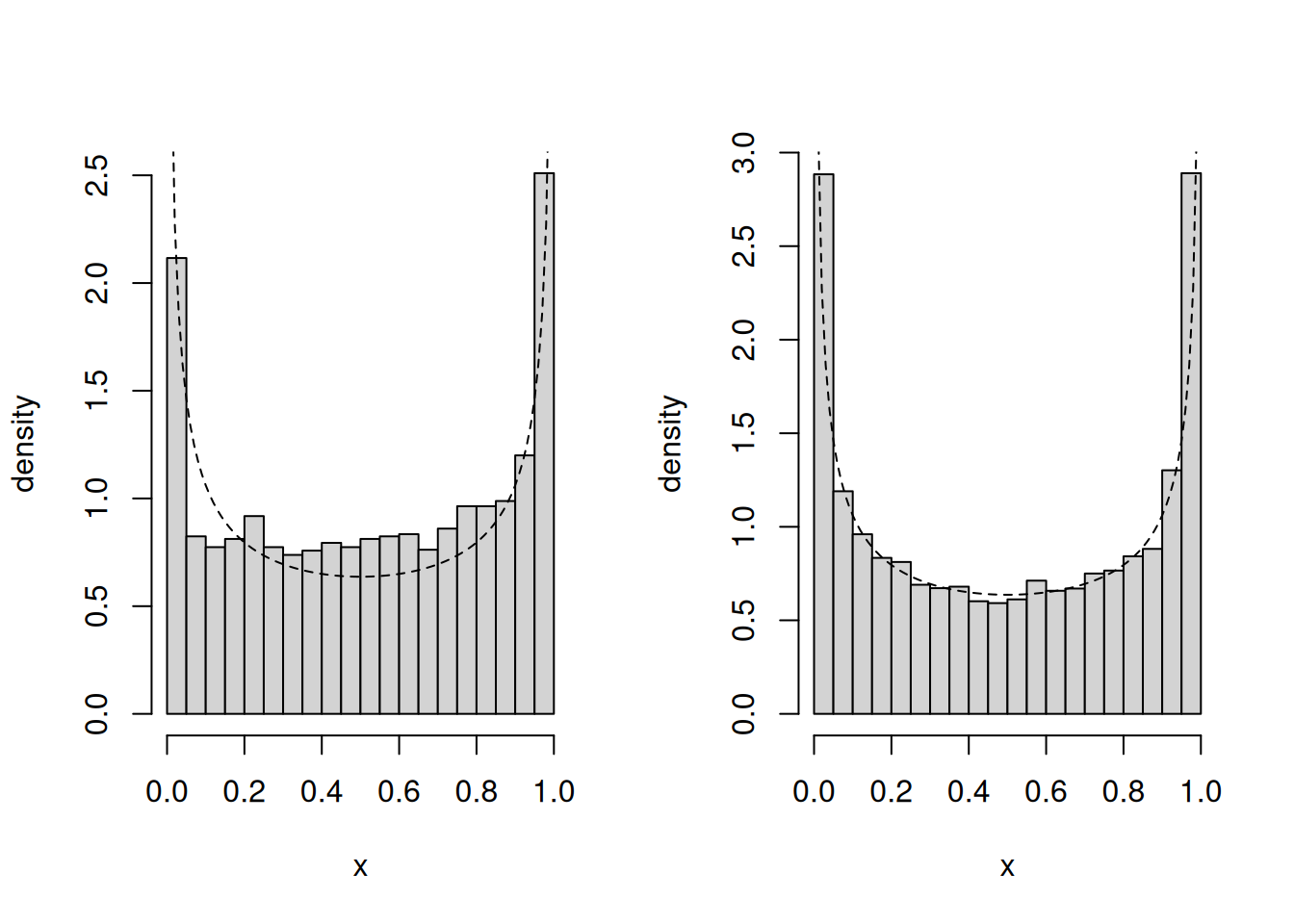
Exercise 5.3
Repeat the simulations in Example 3.6, this time with a parametrization in terms of log rates \(\lambda_i\) \((i=1,2)\), with the same priors. Use a Metropolis–Hastings algorithm with a Gaussian random walk proposal, updating parameters one at a time. Run four chains in parallel.
- Tune the variance to reach an approximate acceptance rate of 0.44.
- Produce diagnostic plots (scatterplots of observations, marginal density plots, trace plots and correlograms). See
bayesplotorcoda. Comment on the convergence and mixing of your Markov chain Monte Carlo. - Report summary statistics of the chains.
Solution. The only thing we need to do is change the parametrization, and add tuning of the variance.
data(upworthy_question, package = "hecbayes")
# Compute sufficient statistics
data <- upworthy_question |>
  dplyr::group_by(question) |>
  dplyr::summarize(ntot = sum(impressions),
                   y = sum(clicks))
# Code log posterior as sum of log likelihood and log prior
loglik <- function(par, counts = data$y, offset = data$ntot, ...){
  lambda <- exp(c(par[1] + log(offset[1]), par[2] + log(offset[2])))
 sum(dpois(x = counts, lambda = lambda, log = TRUE))
}
logprior <- function(par, ...){
  sum(dnorm(x = par, mean = log(0.01), sd = 1.5, log = TRUE))
}
logpost <- function(par, ...){
  loglik(par, ...) + logprior(par, ...)
}
# Compute maximum a posteriori (MAP)
map <- optim(
  par = rep(-4, 2),
  fn = logpost,
  control = list(fnscale = -1),
  offset = data$ntot,
  counts = data$y,
  hessian = TRUE)
# Use MAP as starting value
cur <- map$par
# Compute logpost_cur - we can keep track of this to reduce calculations
logpost_cur <- logpost(cur)
# Proposal covariance
cov_map <- -2*solve(map$hessian)
chol <- chol(cov_map)

set.seed(80601)
niter <- 1e4L
nchains <- 4L
npar <- 2L
chain <- array(0, dim = c(niter, nchains, npar))
naccept <- 0L
for(j in 1:nchains){
  for(i in seq_len(niter)){
    # Multivariate normal proposal - symmetric random walk
    prop <- chol %*% rnorm(n = 2)/1.05 + cur
    logpost_prop <- logpost(prop)
    # Compute acceptance ratio (no q because the ratio is 1)
    logR <- logpost_prop - logpost_cur
    if(logR > -rexp(1)){
      cur <- prop
      logpost_cur <- logpost_prop
      naccept <- naccept + 1L
    }
    chain[i,j,] <- cur
  }
}
# Acceptance rate
naccept/(nchains * niter)
[1] 0.44355# Create some summary graphs
library(bayesplot)
# Name chains so that the graphs can be labelled
dimnames(chain)[[3]] <- c("lambda[1]","lambda[2]")
# Trace plots, correlograms, density plots and bivariate scatterplot
bayesplot::mcmc_trace(chain)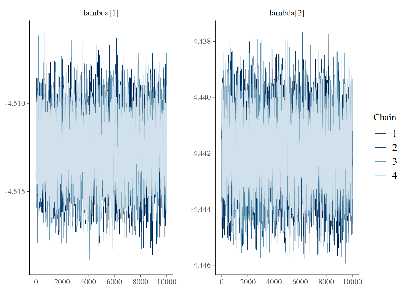
bayesplot::mcmc_acf_bar(chain)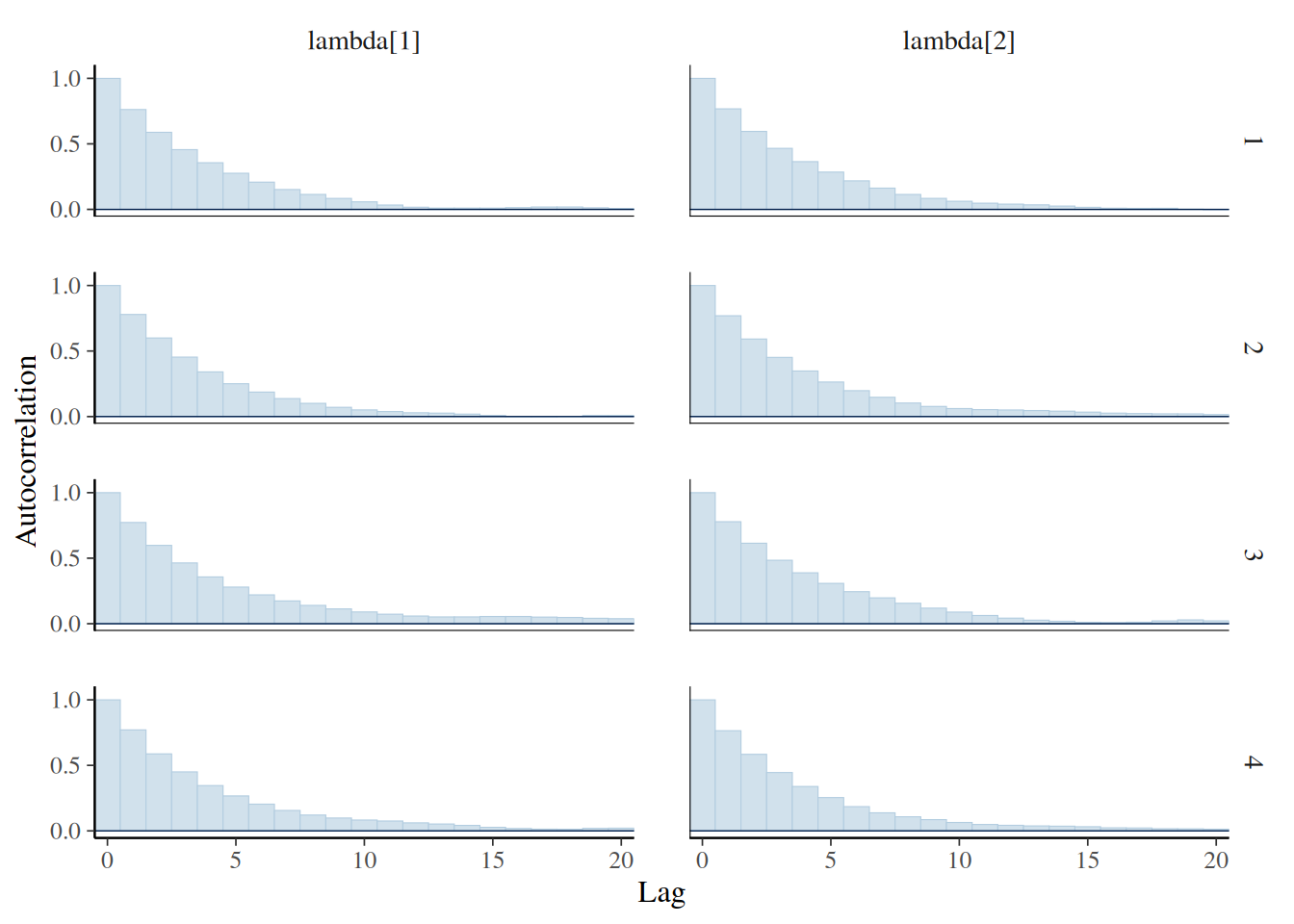
bayesplot::mcmc_dens(chain)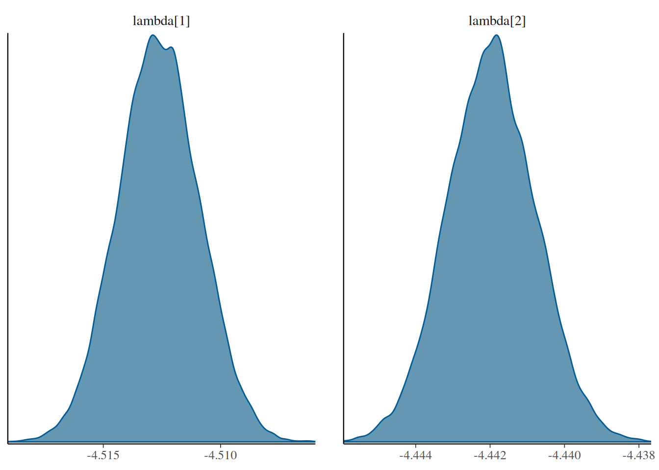
bayesplot::mcmc_scatter(chain)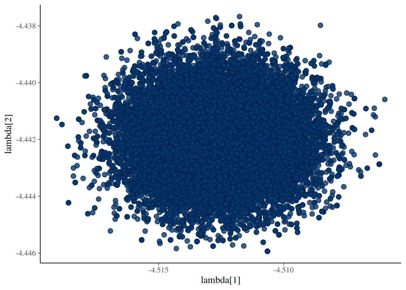
# Posterior summaries with coda
# Need to create a list of mcmc objects...
mcmc_list <- coda::as.mcmc.list(
    lapply(seq_len(nchains),
           function(ch) coda::as.mcmc(chain[, ch, ])))
summary(mcmc_list)
Iterations = 1:10000
Thinning interval = 1
Number of chains = 4
Sample size per chain = 10000

1. Empirical mean and standard deviation for each variable,
   plus standard error of the mean:

            Mean       SD  Naive SE Time-series SE
lambda[1] -4.513 0.001730 8.648e-06      2.384e-05
lambda[2] -4.442 0.001192 5.962e-06      1.670e-05

2. Quantiles for each variable:

            2.5%    25%    50%    75%  97.5%
lambda[1] -4.516 -4.514 -4.513 -4.511 -4.509
lambda[2] -4.444 -4.443 -4.442 -4.441 -4.440