Solution 4

Exercise 4.1

Consider the Laplace family of distribution, \(\mathsf{Laplace}(\nu, \tau)\), with density \[\begin{align*} g(x; \nu, \tau) = \frac{1}{2\tau} \exp\left(- \frac{|x-\nu|}{\tau}\right), \qquad \nu \in \mathbb{R}, \tau > 0 \end{align*}\] as a candidate distribution for rejection sampling from \(\mathsf{Gauss}(0,1)\).

Provide an inversion sampling algorithm to generate from \(\mathsf{Laplace}(\nu, \tau)\).
Can you use the proposal to generate from a standard Gaussian? for Student-\(t\) with 1 degree of freedom? Justify your answer.
Consider as proposal a location-scale version of the Student-t with \(\nu=3\) degrees of freedom. Find the optimal location and scale parameters and the upper bound \(C\) for your choice.
Use the accept-reject to simulate 1000 independent observations and compute the empirical acceptance rate.

Solution.

The distribution function is \[\begin{align*} F(x) = \begin{cases} \frac{1}{2} \exp\left(\frac{x-\nu}{\tau}\right) & x \leq \nu\\ 1 - \frac{1}{2} \exp\left(-\frac{x-\nu}{\tau}\right) & x >\nu\\ \end{cases} \end{align*}\] and using the quantile transform, set \(X=\nu + \tau \log(2U)\) if \(U \leq 0.5\) and \(X=\nu - \tau\log(2-2U)\) if \(U > 0.5\) for \(U \sim \mathsf{unif}(0,1)\).
The Gaussian has lighter tail than the Laplace, so this won’t work. The Cauchy distribution would be a suitable candidate, albeit too heavy tailed.
The optimal value for the location of the Student-\(t\) would be \(\nu\) (here zero for the standard Laplace). We compute the optimal scale via in the code below: \[ \mathrm{argmax}_{\sigma \in \mathbb{R}_{+}}\mathrm{argmin}_{x \in \mathbb{R}} \{\log f(x) - \log g(x; \sigma)\} \]

#' Laplace density
dlaplace <- function(x, loc = 0, scale = 1, log = FALSE){
 stopifnot(scale > 0)
 logdens <-  -log(2*scale) - abs(x-loc)/scale
 if(log){
 return(logdens)
 } else{
 return(exp(logdens))
 }
}
dstudent <- function(x, loc = 0, scale = 1, df = 1, log = FALSE){
  logdens <- -log(scale) + dt(x = (x - loc)/scale, df = df, log = TRUE)
   if(log){
    return(logdens)
   } else{
   return(exp(logdens))
   }
}
# For each value of the scale sigma,
# find the minimum value of x (typically at zero)
opt <- optimize(f = function(sigma){
  optimize(f = function(x){
  dlaplace(x, log = TRUE) - 
    dstudent(x, scale = sigma, df = 3, log = TRUE)}, 
  maximum = TRUE, 
  interval = c(-100, 100))$objective
}, interval = c(0.1,10))
(C <- exp(opt$objective))

[1] 1.261368

(sigma <- opt$minimum)

[1] 0.9272381

# Simulate from accept-reject
ntrials <- 1.1*C*1000
# Simulate from location-scale student
candidate <- sigma*rt(n = ntrials, df = 3)
# Compute log of acceptance rate
logR <- dlaplace(candidate, log = TRUE) - 
  dstudent(candidate, scale = sigma, df = 3, log = TRUE) 
samp <- candidate[logR >= log(C) + -rexp(ntrials)]
# Monte Carlo estimator of the acceptance rate
ntrials/length(samp)

[1] 1.274109

# Plot density
library(ggplot2)
ggplot(data = data.frame(x = samp),
       mapping = aes(x = x)) +
  geom_density() +
  theme_classic()

The Monte Carlo acceptance rate is 1.27, compared with the analytical bound found via numerical optimization of 1.26, to two significant digits.

Exercise 4.2

We revisit Exercise 2.3, which used a half-Cauchy prior for the exponential waiting time of buses.

The ratio-of-uniform method, implemented in the rust R package, can be used to simulate independent draws from the posterior of the rate \(\lambda\). The following code produces

nobs <- 10L # number of observations
ybar <- 8   # average waiting time
B <- 1e4L  # number of draws
# Un-normalized log posterior: scaled log likelihood + log prior
upost <- function(x){ 
  dgamma(x = x, shape = nobs + 1L, rate = nobs*ybar, log = TRUE) +
    log(2) + dt(x = x, df = 1, log = TRUE)}
post_samp <- rust::ru(logf = upost, 
                      n = B, 
                      d = 1,  # dimension of parameter (scalar)
                      init = nobs/ybar)$sim_vals # initial value of mode

Estimate using the independent Monte Carlo samples:

the probability that the average waiting time \(1/\lambda\) is between 3 and 15 minutes
the average waiting time
the standard deviation of the average waiting time.

Next, implement a random walk Metropolis–Hastings algorithm to sample draws from the posterior and re-estimate the quantities. Compare the values.

Solution.

# Monte Carlo for waiting time
# Lambda is the reciprocal mean (1/minute)
times_mc <- 1/post_samp
mean(times_mc > 3 & times_mc < 15)

[1] 0.98

sd(times_mc)

[1] 2.642588

# posterior mean
mean(times_mc)

[1] 7.978362

# Standard error of posterior mean
sd(times_mc)/sqrt(length(post_samp))

[1] 0.02642588

# Metropolis-Hastings algorithm
B <- 1e4L
curr <- 8/10 # prior mean
chains <- numeric(B) # container
sd_prop <- 0.1 # proposal standard deviation
for(b in seq_len(B)){
  prop <- rnorm(n = 1, mean = curr, sd = sd_prop)
  if(upost(prop) - upost(curr) > -rexp(1)){
    curr <- prop
  }
  chains[b] <- curr
}
# Discard burn-in
times <- 1/chains[-(1:100)]
# Estimate quantities using Monte Carlo
mean(times > 3 & times < 15)

[1] 0.9773737

mean(times)

[1] 8.010612

sd(times)

[1] 2.676302

# Summary of MCMC
mcmc <- coda::mcmc(times)
summary(mcmc)


Iterations = 1:9900
Thinning interval = 1 
Number of chains = 1 
Sample size per chain = 9900 

1. Empirical mean and standard deviation for each variable,
   plus standard error of the mean:

          Mean             SD       Naive SE Time-series SE 
       8.01061        2.67630        0.02690        0.05787 

2. Quantiles for each variable:

  2.5%    25%    50%    75%  97.5% 
 4.283  6.170  7.538  9.203 14.691

We can see that the standard error for the mean is roughly twice as big. We would thus need to inflate the sample size by a factor four to get the same precision.

Solution 4.3

Consider the following code which implements a Metropolis–Hastings algorithm to simulate observations from a \(\mathsf{beta}(0.5, 0.5)\) density.

log_f <- function(par){
  dbeta(x = par, shape1 = 0.5, shape2 = 0.5, log = TRUE)
}
metropo <- function(B, sd_prop = 0.2){
  chain <- rep(0, B)
  # Draw initial value
  cur <- runif(1)
  for(b in seq_len(B)){
    repeat {
        # Simulate proposal from Gaussian random walk proposal
        prop <- cur + rnorm(1, sd = sd_prop)
        # check admissibility for probability of success
        if (prop >= 0 & prop <= 1)
          break
    }
    # Compute (log) acceptance ratio
    logR <- log_f(prop) - log_f(cur) 
    # Accept the move if R > u
    if(isTRUE(logR > log(runif(1)))){
     cur <- prop 
    }
    chain[b] <- cur
  }
  return(chain)
}
# Run MCMC for 10K iterations
mc <- metropo(1e4L)

To see if the algorithm works:

Plot the density of the Markov chain draws along with the beta density curve.
Check that empirical moments match the theoretical ones

If the algorithm is incorrect, provide a fix and explain the reason for the problem.

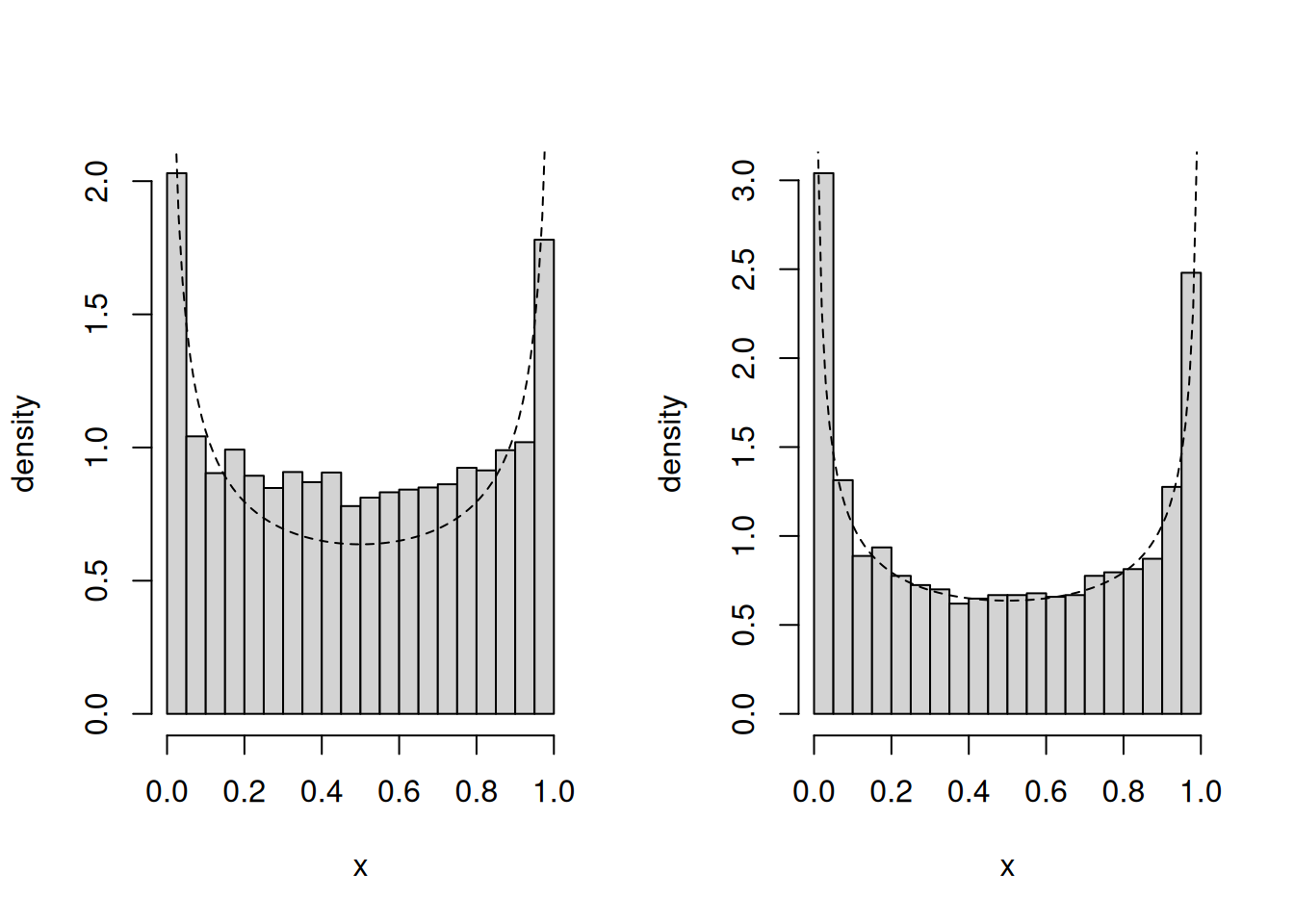
Solution. The sampler is incorrect because it tacitly draws from Gaussian variables that are restricted to \([0,1]\) via the accept-reject step. This means in particular that the acceptance ratio involves constants for the probability given a Gaussian centered at the current value or proposal truncated on the unit interval \[\frac{q(x^{\text{cur}\hphantom{c}} \mid x^{\text{prop}})}{q(x^{\text{prop}} \mid x^{\text{cur}\hphantom{c}})} = \frac{\Phi\{(1-x^{\text{cur}})/\sigma^{\text{prop}}\} - \Phi(-x^{\text{cur}}/\sigma^{\text{prop}})}{\Phi\{(1-x^{\text{prop}})/\sigma^{\text{prop}}\} - \Phi(-x^{\text{prop}}/\sigma^{\text{prop}})}.\]

This exercise was inspired by this blog post by Darren Wilkinson.

log_f <- function(par){
  dbeta(x = par, shape1 = 0.5, shape2 = 0.5, log = TRUE)
}
metropo_fixed <- function(B, sd_prop = 0.2){
  chain <- rep(0, B)
  # Draw initial value
  cur <- runif(1)
  for(b in seq_len(B)){
    repeat {
        # Simulate proposal from Gaussian random walk proposal
        prop <- cur + rnorm(1, sd = sd_prop)
        # check admissibility for probability of success
        if (prop >= 0 & prop <= 1)
          break
    }
    # Compute (log) acceptance ratio
    logR <- log_f(prop) - log_f(cur) + 
      log(pnorm(1, mean = cur, sd = sd_prop) - pnorm(0, mean = cur, sd = sd_prop)) -
      log(pnorm(1, mean = prop, sd = sd_prop) - pnorm(0, mean = prop, sd = sd_prop))
    # Accept the move if R > u
    if(isTRUE(logR > log(runif(1)))){
     cur <- prop 
    }
    chain[b] <- cur
  }
  return(chain)
}
# Run MCMC for 10K iterations
mc2 <- metropo_fixed(1e4L)

Figure 1: Comparison of histogram for 10K draws from the incorrect sampler (left) and the correct sampler (right).