#############################################################
## CAVI algorithm for K-components Gaussian mixture models
#############################################################
# Parameters are
# 1) weights w (probability of components)
# 2) cluster means mu
# 3) cluster variance sigma_sq
# 4) binary indicators of clusters "a" (data augmentation)
CAVI_gauss_mixt <- function(K = 2L, y,
                prior_mean_mu = rep(0, K),
                prior_var_mu = rep(1e8, K),
                prior_shape_var = rep(0.01, K),
                prior_rate_var = rep(0.01, K),
                prior_shape_weights = 0.01,
                maxiter = 1000L,
                tol = 1e-8
                ){
  stopifnot(K >= 1)
  K <- as.integer(K)
  n <- length(y)
  # ELBO normalizing constant (only depends on hyperparameters)
lcst <- 0.5*K*(1-n*log(2*pi)) +
  lgamma(K*prior_shape_weights) -
  K*lgamma(prior_shape_weights) -
  lgamma(n + K*prior_shape_weights)  +
  sum(prior_shape_var*log(prior_rate_var)) -
  sum(lgamma(prior_shape_var))
# Initialization
mu <- runif(K)*diff(range(y))
sigma_sq <- alpha <- rep(1, K)
A <- B <- rep(1, K) # K vector
ELBO <- numeric(maxiter)
nu <- matrix(NA, nrow = n, ncol = K)
# CAVI runs
for(b in seq_len(maxiter)){
  for(k in seq_len(K)){
    nu[, k] <- exp(digamma(alpha[k]) + 0.5*digamma(A[k]) - 0.5*log(B[k]) -
                   0.5*A[k]/B[k]*((y-mu[k])^2+ sigma_sq[k]))
  }
  omega <- nu/rowSums(nu) # Probability of components for each obs
  om <- colSums(omega) # sample size in each cluster
  sigma_sq <- 1/(1/prior_var_mu + A*om/B) # posterior variance of cluster
  mu <- sigma_sq*(prior_mean_mu/prior_var_mu + A/B*colSums(omega * y)) # posterior mean of cluster
  alpha <- prior_shape_weights + om
  A <- prior_shape_var + 0.5*om
  B <- prior_rate_var + 0.5*(colSums(omega*(outer(y, mu, FUN = "-")^2)) + om*sigma_sq)
  # Compute ELBO
  ELBO[b] <- lcst + sum(lgamma(A) - A*log(B) +
    lgamma(alpha) + 0.5*(log(sigma_sq) - log(prior_var_mu)) -
    0.5*((mu-prior_mean_mu)^2 + sigma_sq)/prior_var_mu) -
    sum(omega*log(omega+1e-80))
  if(b >=2){
    if((ELBO[b]-ELBO[b-1]) < tol){
      break
    }
  }
}
list(elbo = ELBO[1:b],
     mu_mean = mu,
     mu_var = sigma_sq,
     sigmasg_shape = A,
     sigmasg_rate = B,
     weights_alpha = alpha,
     probs = omega,
     mean_probs = alpha/sum(alpha),
     cluster_probs = colSums(omega)/sum(omega)
)
}Solution 10
Exercise 10.1
Suppose that \(p(\boldsymbol{\theta})\) is a density with \(\boldsymbol{\theta} \in \mathbb{R}^d\) and that we consider a Gaussian approximation \(q(\boldsymbol{\theta})\) with mean \(\boldsymbol{\mu}\) and covariance matrix \(\boldsymbol{\Sigma}\). Show that the parameters that minimize the Kullback–Leibler \(\mathsf{KL}\{p(\boldsymbol{\theta} \parallel q(\boldsymbol{\theta})\}\) are the expectation and variance under \(p(\boldsymbol{\theta})\).1
Solution. Refer to the Matrix cookbook
Consider \(g \equiv \phi_d(\cdot; \boldsymbol{\mu},\boldsymbol{\Sigma})\) a Gaussian density and \(p(\boldsymbol{\theta})\) the target. Optimization of the parameters of \(g\) can be performed by differentiation of the target. The Kullback–Leibler divergence involves two terms: the negative entropy, which is constant, and the expected value of log density, so \[\begin{align*} \mathsf{KL}(p \parallel g) \stackrel{\boldsymbol{\mu}, \boldsymbol{\Sigma}}{\propto} -\frac{1}{2} \mathsf{E}_{p}\left\{ (\boldsymbol{\theta}-\boldsymbol{\mu})^\top\boldsymbol{\Sigma}^{-1}(\boldsymbol{\theta}-\boldsymbol{\mu})\right\} - \frac{1}{2} \log |\boldsymbol{\Sigma}| \end{align*}\] Taking gradients (formulas 57 and 61 of the Matrix Cookbook) and interchanging the order of integration and differentiation, assuming that the first two moments of \(p(\boldsymbol{\theta})\) exists, gives \[\begin{align*} \frac{\partial}{\partial \boldsymbol{\mu}} \mathsf{KL}(p \parallel g) &= \mathsf{E}_{p}\left\{(\boldsymbol{\theta}-\boldsymbol{\mu})^\top\right\}\boldsymbol{\Sigma}^{-1} \\ \frac{\partial}{\partial \boldsymbol{\Sigma}} \mathsf{KL}(p \parallel g) &= \frac{1}{2} \boldsymbol{\Sigma}^{-1} \mathsf{E}_{p}\left\{(\boldsymbol{\theta}-\boldsymbol{\mu})(\boldsymbol{\theta}-\boldsymbol{\mu})^\top\right\}\boldsymbol{\Sigma}^{-1} - \frac{1}{2}\boldsymbol{\Sigma}^{-1} \end{align*}\] Equating these to zero yields \(\mathsf{E}_p(\boldsymbol{\theta}) = \boldsymbol{\mu}\) and \(\mathsf{E}_p\left\{(\boldsymbol{\theta}-\boldsymbol{\mu})(\boldsymbol{\theta}-\boldsymbol{\mu})^\top\right\} = \boldsymbol{\Sigma}\) provided \(\boldsymbol{\Sigma}\) is invertible.
Exercise 10.2
Consider a finite mixture model of \(K\) univariate Gaussian \(\mathsf{Gauss}(\mu_k, \tau_k^{-1})\) with \(K\) fixed, whose density is \[\begin{align*} \sum_{k=1}^{K} w_k \left(\frac{\tau_k}{2\pi}\right)^{1/2}\exp \left\{-\frac{\tau_k}{2}(y_i-\mu_k)^2\right\} \end{align*}\] where \(\boldsymbol{w} \in \mathbb{S}_{K-1}\) are positive weights that sum to one, meaning \(w_1 + \cdots + w_K=1.\) We use conjugate priors \(\mu_k \sim \mathsf{Gauss}(0, 100)\), \(\tau_k \sim \mathsf{Gamma}(a, b)\) for \(k=1, \ldots, K\) and \(\boldsymbol{w} \sim \mathsf{Dirichlet}(\alpha)\) for \(a, b, \alpha>0\) fixed hyperparameter values.
To help with inference, we introduce auxiliary variables \(\boldsymbol{U}_1, \ldots, \boldsymbol{U}_n\) where \(\boldsymbol{U}_i \sim \mathsf{multinom}(1, \boldsymbol{w})\) that indicates which cluster component the model belongs to, and \(w_k = \Pr(U_{ik}=1).\)
The parameters and latent variables for the posterior of interest are \(\boldsymbol{\mu}, \boldsymbol{\tau}, \boldsymbol{w}\) and \(\boldsymbol{U}.\) Consider a factorized decomposition in which each component is independent of the others, \(g_{\boldsymbol{w}}(\boldsymbol{w})g_{\boldsymbol{\mu}}(\boldsymbol{\mu})g_{\boldsymbol{\tau}}(\boldsymbol{\tau}) g_{\boldsymbol{U}}(\boldsymbol{u}).\)
- Apply the coordinate ascent algorithm to obtain the distribution for the optimal components.
- Write down an expression for the ELBO.
- Run the algorithm for the
geyserdata fromMASSR package for \(K=2\) until convergence with \(\alpha=0.1, a=b=0.01.\) Repeat multiple times with different initializations and save the ELBO for each run. - Repeat these steps for \(K=2, \ldots, 6\) and plot the ELBO as a function of \(K\). Comment on the optimal number of cluster components suggested by the approximation to the marginal likelihood.
Solution.
Code
# Fit the model
data(geyser, package = "MASS")
mixt <- CAVI_gauss_mixt(K = 2, y = geyser$duration)
plot(mixt$elbo,
     xlab = "number of iterations",
     ylab = "evidence lower bound",
     type = "b")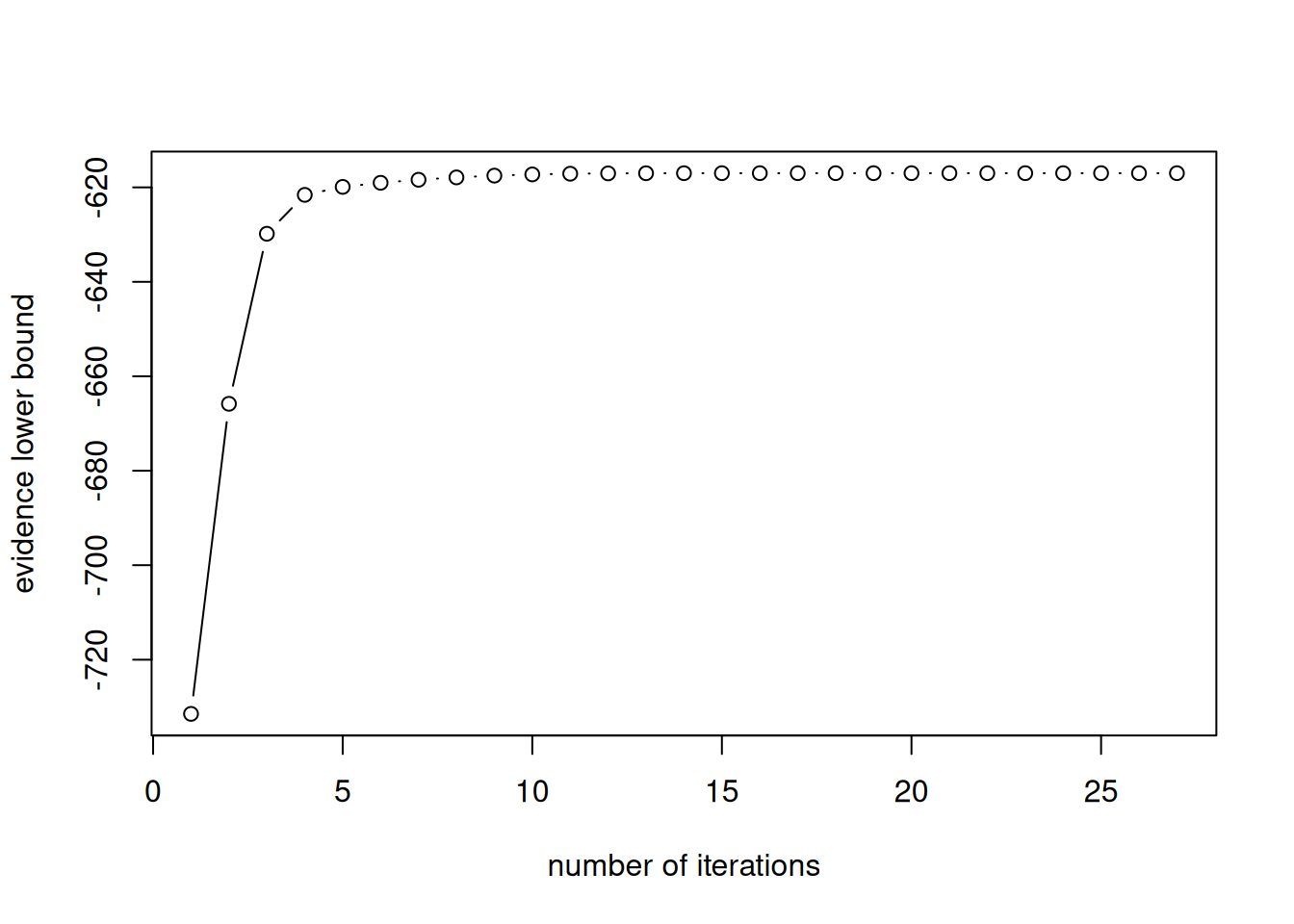
Code
# Compute posterior mean of mean, variance and probability of each cluster
post_prob <- mixt$mean_probs
post_mean <- mixt$mu_mean
post_sd <- sqrt(mixt$sigmasg_rate/(mixt$sigmasg_shape-1))
# Plot the mixture density at posterior mean
curve(post_prob[1]*dnorm(x, mean = post_mean[1], sd = post_sd[1]) +
        post_prob[2]*dnorm(x, mean = post_mean[2], sd = post_sd[2]),
      from = 1,
      to = 6,
      n = 1001,
      xlab = "duration of geyser eruption (in minutes)",
      ylab = "density")
rug(geyser$duration)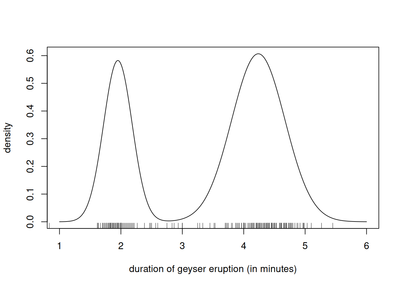
Footnotes
Note that this is not a variational approximation!↩︎