Exercises 6
Exercise 6.1
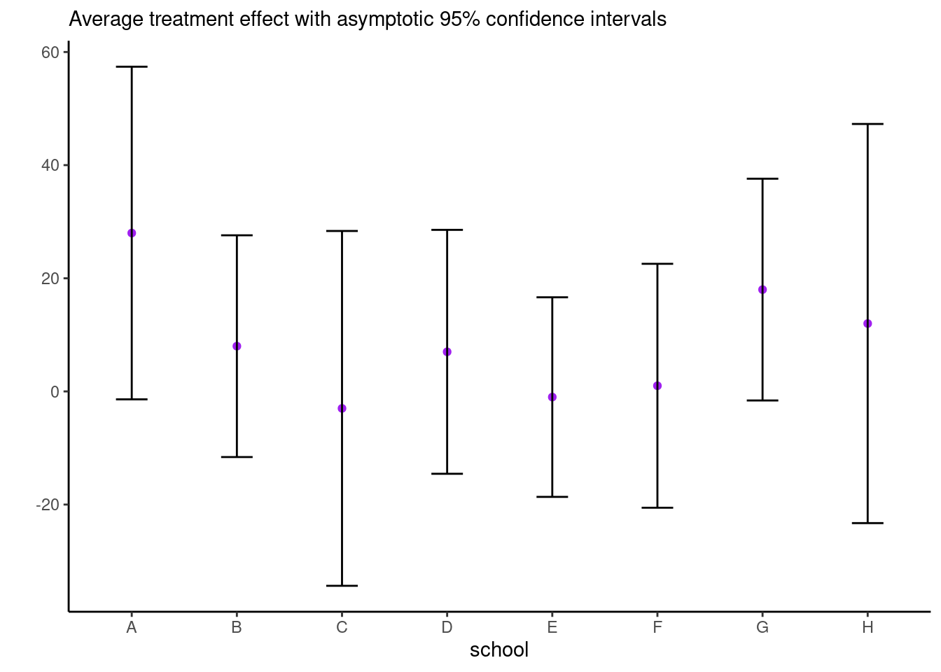
Consider the eight school data from Educational Testing Service (ETS), featured prominently in Gelman et al. (2013). The data shows results of randomized experiments in eight different schools to estimate the effect of coaching on SAT-V scores. The data consist of estimated treatment mean difference and their standard errors. The data size are large, so the average treatment effect (ATE) can be considered Gaussian and the standard errors are treated as a known quantity.
Consider a one-way ANOVA with a single observation per group, where for \(i=1, \ldots, n,\) we have \[\begin{align*} Y_{i} &\sim \mathsf{Gauss}(\mu + \alpha_i, \sigma^2_i) \\ \alpha_i &\sim \mathsf{Gauss}(0, \sigma^2_\alpha) \end{align*}\] and an improper prior for the mean \(p(\mu) \propto 1.\) If there are \(K\) groups, then the group-specific mean is \(\mu+\alpha_k\), and there is a redundant parameter. In the Bayesian setting, the parameters are weakly identifiable because of the prior on \(\boldsymbol{\alpha}\), but the geometry is such that \(\alpha_k \to 0\) as \(\sigma^2_{\alpha} \to 0.\) See Section 5.5 on p. 119 of Gelman et al. (2013) for more details.
We fit the model by adding redundant parameter to improve mixing (Gelman et al., 2008) \[\begin{align*} Y_{i} &\sim \mathsf{Gauss}(\mu + \alpha\xi_i, \sigma^2_i) \\ \xi_i &\sim \mathsf{Gauss}(0, \sigma^2_\xi) \end{align*}\] so that \(\sigma_\alpha = |\alpha|\sigma_\xi.\)
# Eight school data
es <- data.frame(school = LETTERS[1:8],
                 y = c(28, 8, -3, 7, -1, 1, 18, 12),
                 se = c(15, 10, 16, 11, 9, 11, 10, 18))
Derive the Gibbs sampler for the two models with improper priors. Note that, to sample jointly from \(p(\mu, \boldsymbol{\alpha} \mid \boldsymbol{y}, \sigma^2_{\alpha}, \boldsymbol{\sigma}^2_{\boldsymbol{y}})\), you can draw from the marginal of \(\boldsymbol{\alpha}\), then the conditional \(\mu \mid \boldsymbol{\alpha}, \cdots\).
Fit the three algorithms described in Gelman et al. (2008) and compare their efficiency via effective sample size (ESS). In particular, draw traceplots and calculate effective sample sizes for
- \(\mu\)
- \(\alpha_1\),
- the sum \(\mu + \alpha_1\).
as well as pairs plot of \(\alpha_i, \log \sigma_{\alpha}\). The latter should display a very strong funnel.
See this post for display of the pathological behaviour that can be captured by divergence in Hamiltonian Monte Carlo.
Exercise 6.2
Let \(Y_{ij1}\) (\(Y_{ij2}\)) denote the score of the home (respectively visitor) team for a soccer match opposing teams \(i\) and \(j\). Maher (1982) suggested modelling the scores as \[\begin{align*} Y_{ij1} \mid \delta, \alpha_i, \beta_j &\sim \mathsf{Poisson}\{\exp(\delta + \alpha_i +\beta_j)\}, \\ Y_{ij2} \mid \delta, \alpha_j, \beta_i &\sim \mathsf{Poisson}\{\exp(\alpha_j+\beta_i)\}, \end{align*}\] where
- \(\alpha_i\) represent the offensive strength of the team,
- \(\beta_j\) the defensive strength of team \(j\) and
- \(\delta\) is the common home advantage.
The scores in a match and between matches are assumed to be conditionally independent of one another given \(\boldsymbol{\alpha}, \boldsymbol{\beta}, \delta\). The data set efl contains the results of football (soccer) matches for the 2015 season of the English Premier Ligue (EPL) and contains the following variables
score: number of goals ofteamduring a matchteam: categorical variable giving the name of the team which scored the goalsopponent: categorical variable giving the name of the adversaryhome: binary variable, 1 ifteamis playing at home, 0 otherwise.
- Specify penalized complexity priors for the regression parameters scale \(\sigma\) that shrink \(\alpha_i \sim \mathsf{Gauss}(0, \sigma^2)\) and \(\beta_j \sim \mathsf{Gauss}(0, \sigma^2)\) to zero, with a probability of 1% of exceeding 1.
- Fit the model and answer the following questions:
- Using the posterior distribution, give the expected number of goals for a match between Manchester United (at home) against Liverpool.
- Report and interpret the estimated posterior mean home advantage \(\widehat{\delta}\).
- Calculate the probability that the home advantage \(\delta\) is positive?
- Comment on the adequacy of the fit by using a suitable statistic for the model fit (e.g. the deviance statistic
- Maher also suggested more complex models, including one in which the offensive and defensive strength of each team changed depending on whether they were at home or visiting another team, i.e. \[\begin{align} Y_{ij1} \sim \mathsf{Poisson}\{\exp(\alpha_i +\beta_j + \delta)\}, Y_{ij2} \sim \mathsf{Poisson}\{\exp(\gamma_j+\omega_i)\}, \end{align}\] Does the second model fit significantly better than than the first? Compare the models using WAIC and Bayes factors.