This chapter reviews some basic notions of probability and statistics that are normally covered in undergraduate or college.
Population and samples
Statistics is the science of uncertainty quantification: of paramount importance is the notion of randomness. Generally, we will seek to estimate characteristics of a population using only a sample (a sub-group of the population of smaller size).
The population of interest is a collection of individuals which the study targets. For example, the Labour Force Survey (LFS) is a monthly study conducted by Statistics Canada, who define the target population as “all members of the selected household who are 15 years old and older, whether they work or not.” Asking every Canadian meeting this definition would be costly and the process would be long: the characteristic of interest (employment) is also a snapshot in time and can vary when the person leaves a job, enters the job market or become unemployed.
In general, we therefore consider only samples to gather the information we seek to obtain. The purpose of statistical inference is to draw conclusions about the population, but using only a share of the latter and accounting for sources of variability. George Gallup made this great analogy between sample and population:
One spoonful can reflect the taste of the whole pot, if the soup is well-stirred
A sample is a random sub-group of individuals drawn from the population. Creation of sampling plans is a complex subject and semester-long sampling courses would be required to evens scratch the surface of the topic. Even if we won’t be collecting data, keep in mind the following information: for a sample to be good, it must be representative of the population under study. Selection bias must be avoided, notably samples of friends or of people sharing opinions.
Because the individuals are selected at random to be part of the sample, the measurement of the characteristic of interest will also be random and change from one sample to the next. However, larger samples of the same quality carry more information and our estimator will be more precise. Sample size is not guarantee of quality, as the following example demonstrates.
Example 1.1 (Polling for the 1936 USA Presidential Election) The Literary Digest surveyed 10 millions people by mail to know voting preferences for the 1936 USA Presidential Election. A sizeable share, 2.4 millions answered, giving Alf Landon (57%) over incumbent President Franklin D. Roosevelt (43%). The latter nevertheless won in a landslide election with 62% of votes cast, a 19% forecast error. Biased sampling and differential non-response are mostly responsible for the error: the sampling frame was built using “phone number directories, drivers’ registrations, club memberships, etc.”, all of which skewed the sample towards rich upper class white people more susceptible to vote for the GOP.
In contrast, Gallup correctly predicted the outcome by polling (only) 50K inhabitants. Read the full story here.
Variable type
- a variable represents a characteristic of the population, for example the sex of an individual, the price of an item, etc.
- an observation is a set of measures (variables) collected under identical conditions for an individual or at a given time.
The choice of statistical model and test depends on the underlying type of the data collected. There are many choices: quantitative (discrete or continuous) if the variables are numeric, or qualitative (binary, nominal, ordinal) if they can be described using an adjective; I prefer the term categorical, which is more evocative.
Most of the models we will deal with are so-called regression models, in which the mean of a quantitative variable is a function of other variables, termed explanatories. There are two types of numerical variables
- a discrete variable takes a finite or countable number of values, prime examples being binary variables or count variables.
- a continuous variable can take (in theory) an infinite possible number of values, even when measurements are rounded or measured with a limited precision (time, width, mass). In many case, we could also consider discrete variables as continuous if they take enough distinct values (e.g., money).
Categorical variables take only a finite of values. They are regrouped in two groups,
- nominal if there is no ordering between levels (sex, color, country of origin) or
- ordinal if they are ordered (Likert scale, salary scale) and this ordering should be reflected in graphs or tables.
We will bundle every categorical variable using arbitrary encoding for the levels: for modelling, these variables taking \(K\) possible values (or levels) must be transformed into a set of \(K-1\) binary 0/1 variables, the omitted level corresponding to a baseline. Failing to declare categorical variables in your favorite software is a common mistake, especially when these are saved in the database using integers rather than strings.
Random variable
Suppose we wish to describe the behaviour of a stochastic phenomenon. To this effect, one should enumerate the set of possible values taken by the variable of interest and their probability: this is what is encoded in the distribution.
Random variables are denoted using capital letters: for example \(Y \sim \mathsf{normal}(\mu, \sigma^2)\) indicates that \(Y\) follows a normal distribution with parameters \(\mu\) and \(\sigma>0.\) If the values of the latter are left unspecified, we talk about the family of distributions. When the values are given, for example \(\mu=0\) and \(\sigma=1\), we deal with a single distribution for which a function encode the probability of the underlying variable.
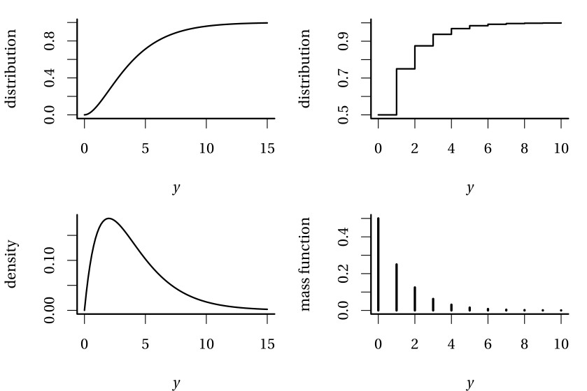
Definition 1.1 (Distribution function, mass function and density) The (cumulative) distribution function \(F(y)\) gives the cumulative probability that an event doesn’t exceed a given numerical value \(y\), \(F(y) = \mathsf{Pr}(Y \leq y).\)
If \(Y\) is discrete, then it has atoms of non-zero probability and we call \(f\) the mass function, and \(f(y)=\mathsf{Pr}(Y=y)\) gives the probability of each outcome \(y.\) In the continuous case, no numerical value has non-zero probability and so we consider intervals instead. The density function \(f(x)\) is non-negative and satisfies \(\int_{\mathbb{R}} f(x) \mathrm{d}x=1\): the integral over a set \(B\) (the area under the curve) gives the probability of \(Y\) falling inside \(B \in \mathbb{R}.\) It follows that the distribution function of a continuous random variable is simply \(F(y) = \int_{-\infty}^y f(x) \mathrm{d} x.\)
One of the first topics covered in introductory statistics is descriptive statistics such as the mean and standard deviation. These are estimators of (centered) moments, which characterise a random variable. In the case of the standard normal distribution, the expectation and variance fully characterize the distribution.
Definition 1.2 (Moments) Let \(Y\) be a random variable with density (or mass) function \(f(x).\) The expectation (or theoretical mean) of a continuous random variable \(Y\) is \[\begin{align*}
\mathsf{E}(Y)=\int_{\mathbb{R}} x f(x) \mathrm{d} x.
\end{align*}\] In the discrete case, we set rather \(\mu = \mathsf{E}(Y)=\sum_{x \in \mathcal{X}} x \mathsf{Pr}(X=x)\), where \(\mathcal{X}\) denotes the support of \(Y\), the set of numerical values at which the probability of \(Y\) is non-zero. More generally, we can look at the expectation of a function \(g(x)\) for \(Y\), which is nothing but the integral (or sum in the discrete case) of \(g(x)\) weighted by the density or mass function of \(f(x),\) meaning \(\int_{\mathbb{R}} g(x) f(x) \mathrm{d} x.\) In the same fashion, provided the integral is finite, the variance is \[\begin{align*}
\mathsf{Va}(Y)=\mathsf{E}\{Y-\mathsf{E}(Y)\}^2 \equiv \int_{\mathbb{R}} (x-\mu)^2 f(x) \mathrm{d} x.
\end{align*}\] The standard deviation is the square root of the variance, \(\mathsf{sd}(Y)=\sqrt{\mathsf{Va}(Y)}\): it units are the same as those of \(Y\) and are thus more easily interpreted.
Example 1.2 Consider a discrete random variable \(Y\) giving the sum of two fair dice throws. The expected value of \(g(Y)=Y^2\) is then \[\begin{align*}
\mathsf{E}(Y^2) &= (2^2 + 12^2) \times \frac{1}{36} + (3^2 + 11^2) \times \frac{2}{36} + (4^2 + 10^2) \\&\;\times \frac{3}{36} + (5^2 +9^2) \times \frac{4}{36} + (6^2 + 8^2) \times \frac{5}{36} \\& + 7^2 \times \frac{6}{36}= \frac{329}{6}.
\end{align*}\]
The notion of moments can be extended to higher dimensions. Consider a column vector of size \(n\) \(\boldsymbol{Y}.\) In the regression setting, the response \(\boldsymbol{Y}\) would usually comprise repeated measures on an individual, or even observations from a group of individuals.
The expected value (theoretical mean) of the vector \(\boldsymbol{Y}\) is calculated componentwise, i.e., \[\begin{align*}
\mathsf{E}(\boldsymbol{Y}) &= \boldsymbol{\mu}=
\begin{pmatrix}
\mathsf{E}(Y_1) &
\cdots &
\mathsf{E}(Y_n)
\end{pmatrix}^\top
\end{align*}\] whereas the second moment of \(\boldsymbol{Y}\) is encoded in the \(n \times n\) covariance matrix \[\begin{align*}
\mathsf{Va}(\boldsymbol{Y}) &= \boldsymbol{\Sigma} = \begin{pmatrix} \mathsf{Va}(Y_1) & \mathsf{Co}(Y_1, Y_2) & \cdots & \mathsf{Co}(Y_1, Y_n) \\
\mathsf{Co}(Y_2, Y_1) & \mathsf{Va}(Y_2) & \ddots & \vdots \\
\vdots & \ddots & \ddots & \vdots \\
\mathsf{Co}(Y_n, Y_1) & \mathsf{Co}(Y_n, Y_2) &\cdots & \mathsf{Va}(Y_n)
\end{pmatrix}
\end{align*}\] The \(i\)th diagonal element of \(\boldsymbol{\Sigma}\), \(\sigma_{ii}=\sigma_i^2\), is the variance of \(Y_i\), whereas the off-diagonal entries \(\sigma_{ij}=\sigma_{ji}\) \((i \neq j)\) are the covariance of pairwise entries, with \[\begin{align*}
\mathsf{Co}(Y_i, Y_j) = \int_{\mathbb{R}^2} (y_i-\mu_i)(y_j-\mu_j) f_{Y_i, Y_j}(y_i, y_j) \mathrm{d} y_i \mathrm{d} y_j.
\end{align*}\] The covariance matrix \(\boldsymbol{\Sigma}\) is thus symmetric. It is customary to normalize the pairwise dependence so they do not depend on the component variance. The linear correlation between \(Y_i\) and \(Y_j\) is \[\begin{align*}
\rho_{ij}=\mathsf{Cor}(Y_i,Y_j)=\frac{\mathsf{Co}(Y_i, Y_j)}{\sqrt{\mathsf{Va}(Y_i)}\sqrt{\mathsf{Va}(Y_j)}}=\frac{\sigma_{ij}}{\sigma_i\sigma_j}.
\end{align*}\] The correlation matrix of \(\boldsymbol{Y}\) is an \(n\times n\) symmetric matrix with ones on the diagonal and the pairwise correlations off the diagonal, \[\begin{align*}
\mathsf{Cor}(\boldsymbol{Y})=
\begin{pmatrix}
1 & \rho_{12} & \rho_{13} & \cdots & \rho_{1n}\\
\rho_{21} & 1 & \rho_{23} & \cdots & \rho_{2n} \\
\rho_{31} & \rho_{32} & 1 & \ddots & \rho_{3n} \\
\vdots & \vdots & \ddots & \ddots & \vdots \\
\rho_{n1} & \rho_{n2} & \rho_{n3} & \cdots & 1
\end{pmatrix}.
\end{align*}\] One of the most important parts of modelling correlated (or longitudinal) data is the need to account for within-group correlations. This basically comes down to modelling a covariance matrix for observations within the same group (or within the same individual in the case of repeated measures), which is the object of Chapter 5.
Definition 1.3 (Pearson linear correlation) The linear correlation between random variables \(X_j\) and \(X_k\), denoted \(r_{j, k}\), measures the strength of the linear relationship between the two variables, i.e., it measures how close the observations are from a line. The sample correlation coefficient is \[\begin{align*}
r_{j, k} &= \frac{\widehat{\mathsf{Co}}(X_j, X_k)}{\{\widehat{\mathsf{Va}}(X_j) \widehat{\mathsf{Va}}(X_k)\}^{1/2}}
%\\&=\frac{\sum_{i=1}^n (x_{i, j}-\overline{x}_j)(x_{i, k} -\overline{x}_{k})}{\left\{\sum_{i=1}^n (x_{i, j}-\overline{x}_j)^2 \sum_{i=1}^n(x_{i, k} -\overline{x}_{k})^2\right\}^{1/2}}
\end{align*}\]
Properties of the linear correlation coefficient \(r\) include:
- \(-1 \leq r \leq 1\);
- \(r=1\) (\(r=-1\)) if and only if the \(n\) observations fall exactly on a positively (negatively) sloped line. In other words, there exist two constants \(a\) and \(b > 0\) \((b <0\)) such that \(y_i=a+b x_i\) for any \(i\).
More generally,
- The sign of the correlation coefficient determines the orientation of the slope (positive of negative).
- The closer the correlation is from 1 (in absolute value), the more the points tend to be aligned.
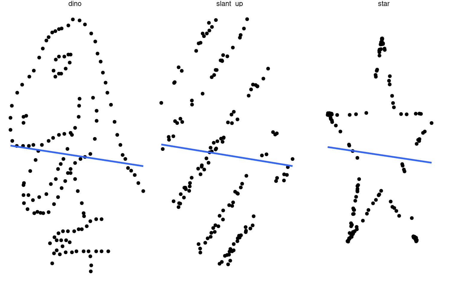
- A correlation of zero does not imply that there is no relationship between the two variables. It only means that there is no linear dependence between the two variables.
Figure 1.1 clearly illustrates the last point: these datasets have near zero linear correlation, and thus the slope is close to flat, but they are not independent since dinosaurs or stars do not arise from independent observations.
Definition 1.4 (Bias) The bias of an estimator \(\hat{\theta}\) for a parameter \(\theta\) is \[\begin{align*}
\mathsf{bias}(\hat{\theta})=\mathsf{E}(\hat{\theta})- \theta
\end{align*}\] The estimator is unbiased if its bias is zero.
Example 1.3 (Unbiased estimators) The unbiased estimator of the mean and the variance of \(Y\) are \[\begin{align*}
\overline{Y}_n &= n^{-1} \sum_{i=1}^n Y_i\\
S_n &= (n-1)^{-1} \sum_{i=1}^n (Y_i-\overline{Y})^2.
\end{align*}\]
While unbiasedness is a desirable property, there may be cases where no unbiased estimator exists for a parameter! Often, rather, we seek to balance bias and variance: recall that an estimator is a function of random variables and thus it is itself random: even if it is unbiased, the numerical value obtained will vary from one sample to the next.
Definition 1.5 We often seek an estimator that minimises the mean squared error, \[\begin{align*}
\mathsf{MSE}(\hat{\theta}) = \mathsf{E}\{(\hat{\theta}-\theta)^2\}=\mathsf{Va}(\hat{\theta}) + \{\mathsf{E}(\hat{\theta})\}^2.
\end{align*}\] The mean squared error is an objective function consisting of the sum of the squared bias and the variance.
Most estimators we will considered are so-called maximum likelihood estimator. These estimator are asymptotically efficient, in the sense that they have the lowest mean squared error of all estimators for large samples. Other properties of maximum likelihood estimators also make them attractive default choice for estimation.
Discrete distributions
Many distributions for discrete random variables have a simple empirical justification, stemming from simple combinatorial arguments (counting). We revisit the most common ones.
Definition 1.6 (Bernoulli distribution) We consider a binary event such as coin toss (heads/tails). In general, the two events are associated with success/failure. By convention, failures are denoted by zeros and successes by ones, the probability of success being \(p\) so \(\mathsf{Pr}(Y=1)=p\) and \(\mathsf{Pr}(Y=0)=1-p\) (complementary event). The mass function of the Bernoulli distribution is thus \[\begin{align*}
\mathsf{Pr}(Y=y) = p^y (1-p)^{1-y}, \quad y=0, 1.
\end{align*}\]
A rapid calculation shows that \(\mathsf{E}(Y)=p\) and \(\mathsf{Va}(Y)=p(1-p).\) Indeed, \[\begin{align*}
\mathsf{E}(Y) = \mathsf{E}(Y^2) = p \cdot 1 + (1-p) \cdot 0 = p.
\end{align*}\]
Many research questions have binary responses, for example:
- did a potential client respond favourably to a promotional offer?
- is the client satisfied with service provided post-purchase?
- will a company go bankrupt in the next three years?
- did a study participant successfully complete a task?
Oftentimes, we will have access to aggregated data.
Definition 1.7 (Binomial distribution) If we consider the sum of independent and identically distributed Bernoulli events, the number of successes \(Y\) out of \(m\) trials is binomial, denoted \(\mathsf{Bin}(m, p)\); the mass function of the binomial distribution is \[\begin{align*}
\mathsf{Pr}(Y=y) = \binom{m}{y}p^y (1-p)^{m-y}, \quad y=0, 1, \ldots, m.
\end{align*}\] The likelihood of a sample from a binomial distribution is (up to a normalizing constant that doesn’t depend on \(p\)) the same as that of \(m\) independent Bernoulli trials. The expectation of the binomial random variable is \(\mathsf{E}(Y)=mp\) and its variance \(\mathsf{Va}(Y)=mp(1-p).\)
As examples, we could consider the number of successful candidates out of \(m\) who passed their driving license test or the number of customers out of \(m\) total which spent more than 10$ in a store.
More generally, we can also consider count variables whose realizations are integer-valued, for examples the number of
- insurance claims made by a policyholder over a year,
- purchases made by a client over a month on a website,
- tasks completed by a study participant in a given time frame.
Definition 1.8 (Poisson distribution) If the probability of success \(p\) of a Bernoulli event is small in the sense that \(mp \to \lambda\) when the number of trials \(m\) increases, then the number of success follows approximately a Poisson distribution with mass function \[\begin{align*}
\mathsf{Pr}(Y=y) = \frac{\exp(-\lambda)\lambda^y}{\Gamma(y+1)}, \quad y=0, 1, 2, \ldots
\end{align*}\] where \(\Gamma(\cdot)\) denotes the gamma function. The parameter \(\lambda\) of the Poisson distribution is both the expectation and the variance of the distribution, meaning \(\mathsf{E}(Y)=\mathsf{Va}(Y)=\lambda.\)
Definition 1.9 (Negative binomial distribution) The negative binomial distribution arises if we consider the number of Bernoulli trials with probability of success \(p\) until we obtain \(m\) success. Let \(Y\) denote the number of failures: the order of success and failure doesn’t matter, except for the latest trial which must be a success. The mass function of the negative binomial is \[\begin{align*}
\mathsf{Pr}(Y=y)= \binom{m-1+y}{y} p^m (1-p)^{y}.
\end{align*}\]
The negative binomial distribution also appears as the unconditional distribution of a two-stage hierarchical gamma-Poisson model, in which the mean of the Poisson distribution is random and follows a gamma distribution. In notation, this is \(Y \mid \Lambda=\lambda \sim \mathsf{Po}(\lambda)\) and \(\Lambda\) follows a gamma distribution with shape \(r\) and scale \(\theta\), whose density is \[\begin{align*}
f(x) = \theta^{-r}x^{r-1}\exp(-x/\theta)/\Gamma(r).
\end{align*}\] The unconditional number of success is then negative binomial.
In the context of generalized linear models, we will employ yet another parametrisation of the distribution, with the mass function \[\begin{align*}
\mathsf{Pr}(Y=y)=\frac{\Gamma(y+r)}{\Gamma(y+1)\Gamma(r)} \left(\frac{r}{r + \mu} \right)^{r} \left(\frac{\mu}{r+\mu}\right)^y, y=0, 1, \ldots, \mu,r >0,
\end{align*}\] where \(\Gamma\) is the gamma function and the parameter \(r>0\) is not anymore integer valued. The expectation and variance of \(Y\) are \(\mathsf{E}(Y)=\mu\) et \(\mathsf{Va}(Y)=\mu+k\mu^2\), where \(k=1/r.\) The variance of the negative binomial distribution is thus higher than its expectation, which justifies the use of the negative binomial distribution for modelling overdispersion.
Continuous distributions
We will encounter many continuous distributions that arise as (asymptotic) null distribution of test statistics because of the central limit theorem, or that follow from transformation of Gaussian random variables.
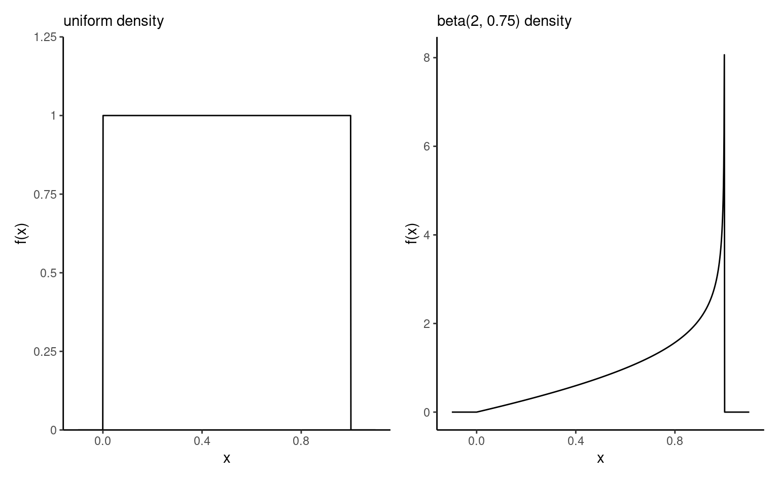
Definition 1.10 (Beta distribution) The beta distribution \(\mathsf{Beta}(\alpha, \beta)\) is a distribution supported on the unit interval \([0,1]\) with shape parameters \(\alpha>0\) and \(\beta>0.\) It’s density is \[\begin{align*}
f(x) = \frac{\Gamma(\alpha)\Gamma(\beta)}{\Gamma(\alpha+\beta)}x^{\alpha-1}(1-x)^{1-\beta}, \qquad x \in [0,1].
\end{align*}\] The case \(\alpha=\beta=1\), also denoted \(\mathsf{unif}(0,1)\), corresponds to a standard uniform distribution.
Definition 1.11 (Exponential distribution) The exponential distribution plays a prominent role in the study of waiting time of Poisson processes, and in survival analysis. One caracteristic of the distribution is it’s absence of memory: \(\Pr(Y \geq y + u \mid Y > u) = \Pr(Y > u)\) for \(y, u>0.\)
The distribution function of the exponential distribution with scale \(\lambda>0\), denoted \(Y \sim \mathsf{Exp}(\lambda)\), is \(F(x) = 1-\exp(-x/\lambda)\) and the corresponding density function is \(f(x) =\lambda^{-1}\exp(-x/\lambda)\) for \(x >0.\) The expected value of \(Y\) is simply \(\lambda.\)
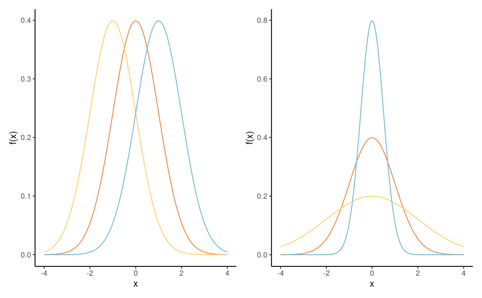
Definition 1.12 (Normal distribution) Ths most well known distribution, the normal distribution is ubiquitous in statistics because of the central limit theorem (CLT), which describes the behaviour of the sample mean in large sample.The parameters \(\mu\) and \(\sigma>0\) that fully characterize the distribution of the normal distribution and they correspond to the expectation and standard deviation. The density of a normal distribution is symmetric around \(\mu\), while \(\sigma\) describes the dispersion around this mode. The bell-shaped density function is \[\begin{align*}
f(x) = (2\pi\sigma^2)^{-1/2} \exp \left\{ - \frac{(x-\mu)^2}{2\sigma^2}\right\}, \qquad x \in \mathbb{R}.
\end{align*}\]
The distribution function of the normal distribution is not available in closed-form. The normal distribution is a location-scale distribution: if \(Y \sim \mathsf{normal}(\mu, \sigma^2)\), then \(Z = (Y-\mu)/\sigma \sim \mathsf{normal}(0,1).\) Conversely, if \(Z \sim \mathsf{normal}(0,1)\), then \(Y = \mu + \sigma Z \sim \mathsf{normal}(\mu, \sigma^2).\)
We will also encounter the multivariate normal distribution; for a \(d\) dimensional vector \(\boldsymbol{Y} \sim \mathsf{normal}_d(\boldsymbol{\mu}, \boldsymbol{\Sigma})\), the density is \[\begin{align*}
f(\boldsymbol{x}) = (2\pi)^{-d/2} |\boldsymbol{\Sigma}|^{-1/2} \exp \left\{ - \frac{1}{2} (\boldsymbol{x}-\boldsymbol{\mu})^\top \boldsymbol{\Sigma}^{-1}(\boldsymbol{x}-\boldsymbol{\mu})\right\}
\end{align*}\]
The mean vector \(\boldsymbol{\mu}\) is the vector of expectation of individual observations, whereas \(\boldsymbol{\Sigma}\) is the \(d \times d\) covariance matrix of \(\boldsymbol{Y}.\) A unique property of the multivariate normal distribution is the link between independence and the covariance matrix: if \(Y_i\) and \(Y_j\) are independent, the \((i,j)\) off-diagonal entry of \(\boldsymbol{\Sigma}\) is zero.
Definition 1.13 (Chi-square distribution) The chi-square distribution with \(\nu>0\) degrees of freedom, denoted \(\chi^2_\nu\) or \(\mathsf{chi-square}(\nu).\) It’s density is \[\begin{align*}
f(x; \nu) = \frac{1}{2^{\nu/2}\Gamma(\nu/2)}x^{\nu/2-1}\exp(-x/2),\qquad x >0.
\end{align*}\] It can be obtained for \(\nu\) integer by considering the following: if we consider \(k\) independent and identically distributed standard normal variables, \(Y_i \sim \mathsf{normal}(0, 1)\), then \(\sum_{i=1}^k Y_i^2\) follows a chi-square distribution with \(k\) degrees of freedom, denote \(\chi^2_k.\) The square of a standard normal variate likewise follows a \(\chi^2_1\) distribution. The expectation of \(\chi^2_k\) random variable is \(k.\)
If we consider a sample of \(n\) normally distributed observations, the scaled sample variance \((n-1)S^2/\sigma^2 \sim \chi^2_{n-1}.\)
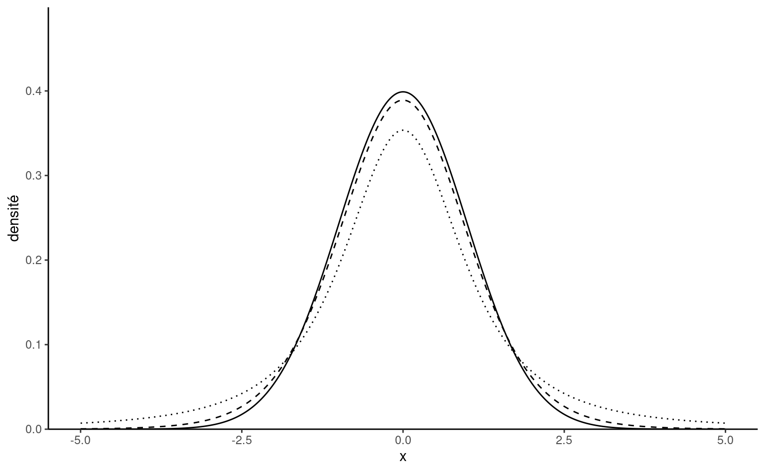
Definition 1.14 (Student-\(t\) distribution) The Student-\(t\) distribution with \(\nu>0\) degrees of freedom is a location-scale family. The standard version is denoted by \(\mathsf{Student}(\nu).\)
The name “Student” comes from the pseudonym used by William Gosset in Gosset (1908), who introduced the asymptotic distribution of the \(t\)-statistic. The density of the standard \(T\) with \(\nu\) degrees of freedom is \[\begin{align*}
f(y; \nu) = \frac{\Gamma \left( \frac{\nu+1}{2}\right)}{\Gamma\left(\frac{\nu}{2}\right)
\sqrt{\nu\pi}}\left(1+\frac{y^{2}}{\nu}\right)^{-\frac{\nu+1}{2}}
\end{align*}\] the distribution has polynomial tails, is symmetric around \(0\) and unimodal. As \(\nu \to \infty\), the Student distribution converges to a normal distribution. It has heavier tails than the normal distribution and only the first \(\nu-1\) moments of the distribution exist, so a Student distribution with \(\nu=2\) degrees of freedom has infinite variance.
For normally distributed data, the centered sample mean divided by the sample variance, \((\overline{Y}-\mu)/S^2\) follows a Student-\(t\) distribution with \(n-1\) degrees of freedom, which explains the terminology \(t\)-tests.
Definition 1.15 (Fisher distribution) The Fisher or \(F\) distribution is used to determine the large sample behaviour of test statistics for comparing different group averages (in analysis of variance) assuming data are normally distributed.
The \(F\) distribution, denoted \(\mathsf{Fisher}(\nu_1, \nu_2)\), is obtained by dividing two independent chi-square random variables with respective degrees of freedom \(\nu_1\) and \(\nu_2.\) Specifically, if \(Y_1 \sim \chi^2_{\nu_1}\) and \(Y_2 \sim \chi^2_{\nu_2}\), then \[\begin{align*}
F = \frac{Y_1/\nu_1}{Y_2/\nu_2} \sim \mathsf{Fisher}(\nu_1, \nu_2)
\end{align*}\]
The Fisher distribution tends to a \(\chi^2_{\nu_1}\) when \(\nu_2 \to \infty.\)
Graphs
This section reviews the main graphical representation of random variables, depending on their type.
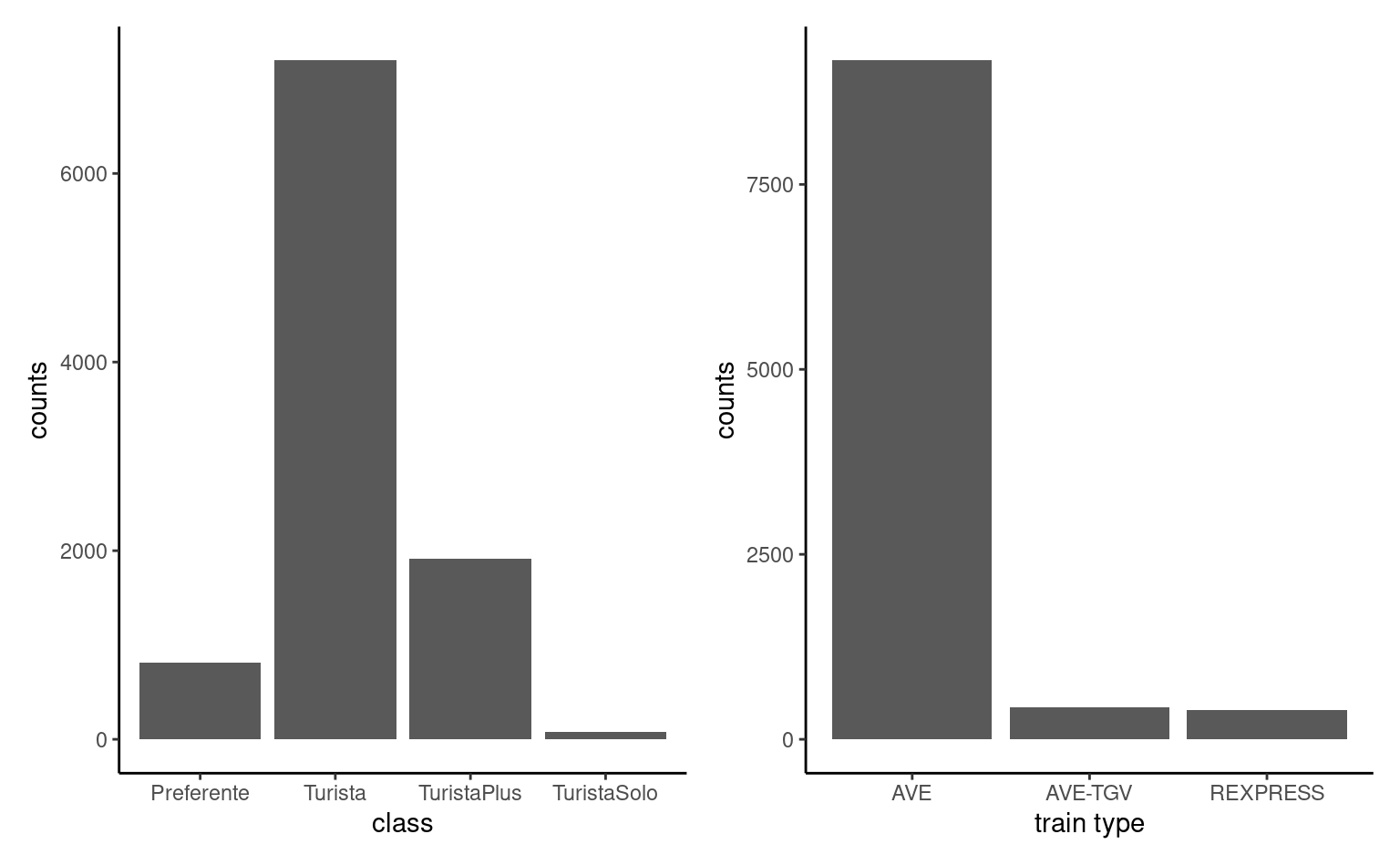
The main type of graph for representing categorical variables is bar plot (and modifications thereof). In a bar plot, the frequency of each category is represented in the \(y\)-axis as a function of the (ordered) levels on the \(x\)-axis. This representation is superior to the ignominious pie chart, a nuisance that ought to be banned (humans are very bad at comparing areas and a simple rotation changes the perception of the graph)!
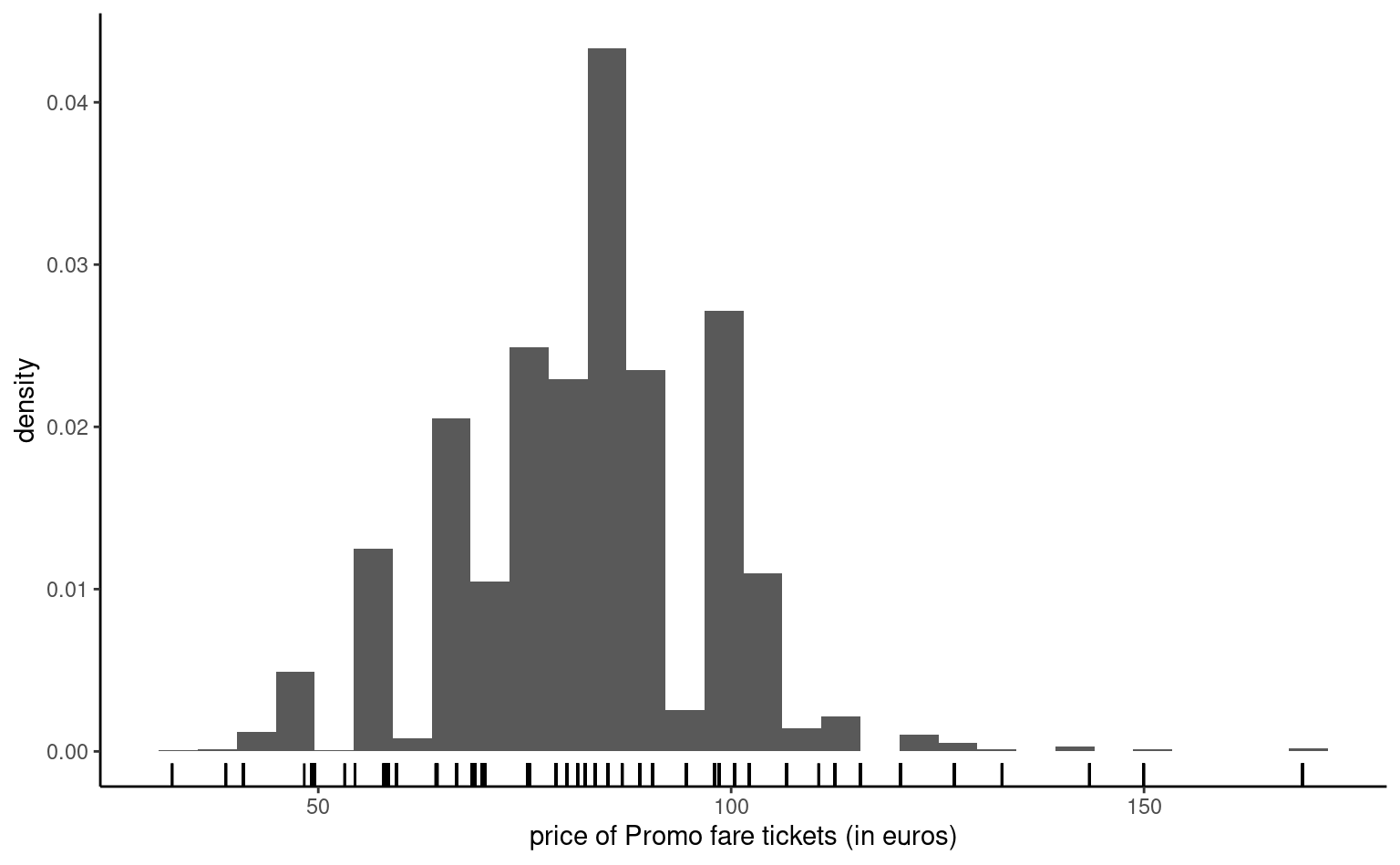
Continuous variables can take as many distinct values as there are observations, so we cannot simply count the number of occurences by unique values. Instead, we bin them into distinct intervals so as to obtain an histogram. The number of class depends on the number of observations: as a rule of thumb, the number of bins should not exceed \(\sqrt{n}\), where \(n\) is the sample size. We can then obtain the frequency in each class, or else normalize the histogram so that the area under the bands equals one: this yields a discrete approximation of the underlying density function. Varying the number of bins can help us detect patterns (rounding, asymmetry, multimodality).
Since we bin observations together, it is sometimes difficult to see where they fall. Adding rugs below or above the histogram will add observation about the range and values taken, where the heights of the bars in the histogram carry information about the (relative) frequency of the intervals.
If we have a lot of data, it sometimes help to focus only on selected summary statistics.
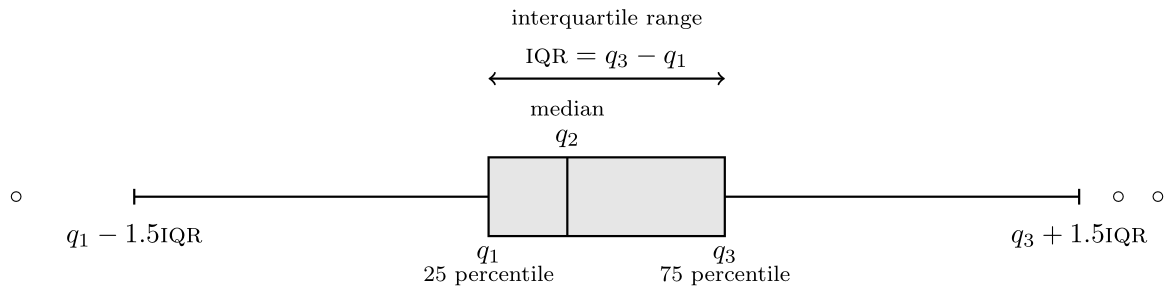
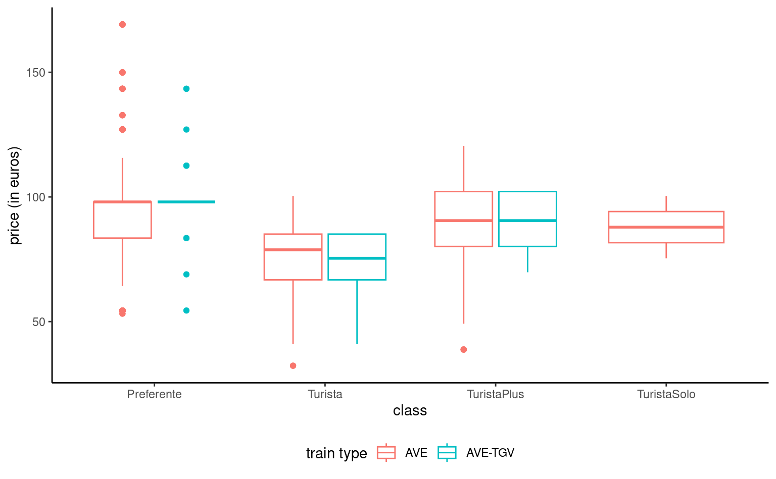
Definition 1.16 (Box-and-whiskers plot) A box-and-whiskers plot (or boxplot) represents five numbers
- The box gives the quartiles \(q_1, q_2, q_3\) of the distribution. The middle bar \(q_2\) is thus the median, so 50% of the observations are smaller or larger than this number.
- The length of the whiskers is up to \(1.5\) times the interquartiles range \(q_3-q_1\) (the whiskers extend until the latest point in the interval, so the largest observation that is smaller than \(q_3+1.5(q_3-q_1)\), etc.)
- Observations beyond the whiskers are represented by dots or circles, sometimes termed outliers. However, beware of this terminology: the larger the sample size, the more values will fall outside the whiskers. This is a drawback of boxplots, which was conceived at a time where the size of data sets was much smaller than what is current standards.
We can represent the distribution of a response variable as a function of a categorical variable by drawing a boxplot for each category and laying them side by side. A third variable, categorical, can be added via a color palette, as shown in Figure 1.8.
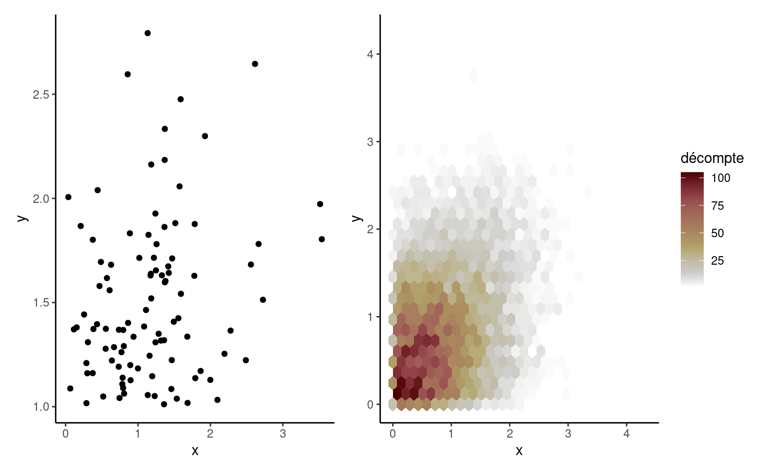
Scatterplots are used to represent graphically the co-variation between two continuous variables: each tuple gives the coordinate of the point. If only a handful of large values are visible on the graph, a transformation may be useful: oftentimes, you will encounter graphs where the \(x\)- or \(y\)-axis is on the log-scale when the underlying variable is positive. If the number of data points is too large, it is hard to distinguish points because they are overlaid: adding transparency, or binning using a two-dimensional histogram with the frequency represented using color are potential solutions. The left panel of Figure 1.9 shows the 100 simulated observations, whereas the right-panel shows a larger sample of 10 000 points using hexagonal binning, an analog of the bivariate density.
Models are (at best) an approximation of the true data generating mechanism and we will want to ensure that our assumptions are reasonable and the quality of the fit decent.
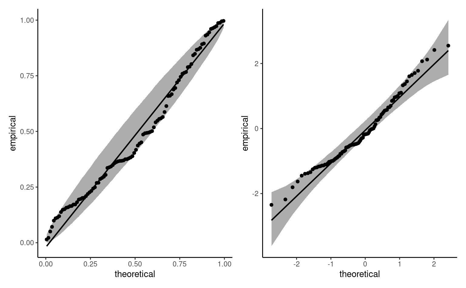
Definition 1.17 (Quantiles-quantiles plots) Quantile-quantile plots are graphical goodness-of-fit diagnostics that are based on the following principle: if \(Y\) is a continuous random variable with distribution function \(F\), then the mapping \(F(Y) \sim \mathsf{unif}(0,1)\) yields standard uniform variables. Similarly, the quantile transform applied to a uniform variable provides a mean to simulating samples from \(F\), viz. \(F^{-1}(U).\) Consider then a random sample of size \(n\) from the uniform distribution ordered from smallest to largest, with \(U_{(1)} \leq \cdots \leq U_{(n)}.\) One can show these ranks have marginally a Beta distribution, \(U_{(k)} \sim \mathsf{beta}(k, n+1-k)\) with expectation \(k/(n+1).\)
In practice, we don’t know \(F\) and, even if we did, one would need to estimate the parameters. We consider some estimator \(\widehat{F}\) for the model and apply the inverse transform to an approximate uniform sample \(\{i/(n+1)\}_{i=1}^n.\) The quantile-quantile plot shows the data as a function of the (first moment) of the transformed order statistics:
- on the \(x\)-axis, the theoretical quantiles \(\widehat{F}^{-1}\{\mathrm{rank}(y_i)/(n+1)\}\)
- on the \(y\)-axis, the empirical quantiles \(y_i\)
If the model is adequate, the ordered values should follow a straight line with unit slope passing through the origin.
Even if we knew the true distribution of the data, the sample variability makes it very difficult to spot if deviations from the model are abnormal or compatible with the model. A simple point estimate with no uncertainty measure can lead to wrong conclusions. As such, we add approximate pointwise or simultaneous confidence intervals. The simplest way to do this is by simulation, by repeating the following steps \(B\) times:
- simulate a sample \(\{Y^{(b)}_{i}\} (i=1,\ldots, n)\) from \(\widehat{F}\)
- re-estimate the parameters of \(F\) to obtain \(\widehat{F}_{(b)}\)
- calculate and save the plotting positions \(\widehat{F}^{-1}_{(b)}\{i/(n+1)\}.\)
The result of this operation is an \(n \times B\) matrix of simulated data. We obtain a symmetric (\(1-\alpha\)) confidence interval by keeping the empirical quantile of order \(\alpha/2\) and \(1-\alpha/2\) from each row. The number \(B\) should be larger than 999, say, and be chosen so that \(B/\alpha\) is an integer.
For the pointwise interval, each order statistic from the sample is a statistic and so the probability of any single one falling outside the confidence interval is approximately \(\alpha.\) However, order statistics are not independent (they are ordered), so its common to see neighbouring points falling outside of their respective intervals. The intervals shown in Figure 1.10 are pointwise and derived (magically) using a simple function. The uniform order statistics have larger variability as we move away from 0.5, but the uncertainty in the quantile-quantile plot largely depends on \(F.\)
Interpretation of quantile-quantile plots requires practice and experience: this post by Glen_b on StackOverflow nicely summarizes what can be detected (or not) from them.
Laws of large numbers
An estimator for a parameter \(\theta\) is consistent if the value obtained as the sample size increases (to infinity) converges to the true value of \(\theta.\) Mathematically speaking, this translates into convergence in probability, meaning \(\hat{\theta} \stackrel{\mathsf{Pr}}{\to} \theta.\) In common language, we say that the probability that \(\hat{\theta}\) and \(\theta\) differ becomes negligible as \(n\) gets large.
Consistency is the a minima requirement for an estimator: when we collect more information, we should approach the truth. The law of large number states that the sample mean of \(n\) (independent) observations with common mean \(\mu\), say \(\overline{Y}_n\), converges to \(\mu\), denoted \(\overline{Y}_n \rightarrow \mu.\) Roughly speaking, our approximation becomes less variable and asymptotically unbiased as the sample size (and thus the quantity of information available for the parameter) increases. The law of large number is featured in Monte Carlo experiments: we can approximate the expectation of some (complicated) function \(g(x)\) by simulating repeatedly independent draws from \(Y\) and calculating the sample mean \(n^{-1} \sum_{i=1}^n g(Y_i).\)
If the law of large number tells us what happens in the limit (we get a single numerical value), the result doesn’t contain information about the rate of convergence and the uncertainty at finite levels.
Central Limit Theorem
The central limit theorem gives the approximate large sample distribution of the sample mean. Consider a random sample of size \(n\) \(\{Y_i\}_{i=1}^n\) of independent random variables with common expectation \(\mu\) and variance \(\sigma^2.\) The sample mean \(\overline{Y} = n^{-1}\sum_{i=1}^n Y_i\) converges to \(\mu\) by the law of large number, but we also have that
- the estimator \(\overline{Y}\) is centered around \(\mu\),
- the standard error is \(\sigma/\sqrt{n}\); the rate of convergence is thus \(\sqrt{n}.\) For a sample of size 100, the standard error of the sample mean will be 10 times smaller than that of the underlying random variable.
- the sample mean, once properly scaled, follows approximately a normal distribution
Mathematically, the central limit theorem states \(\sqrt{n}(\overline{Y}-\mu) \stackrel{\mathrm{d}}{\rightarrow} \mathsf{normal}(0, \sigma^2).\) If \(n\) is large (a rule of thumb is \(n>30\), but this depends on the underlying distribution of \(Y\)), then \(\overline{Y} \stackrel{\cdot}{\sim} \mathsf{normal}(\mu, \sigma^2/n).\)
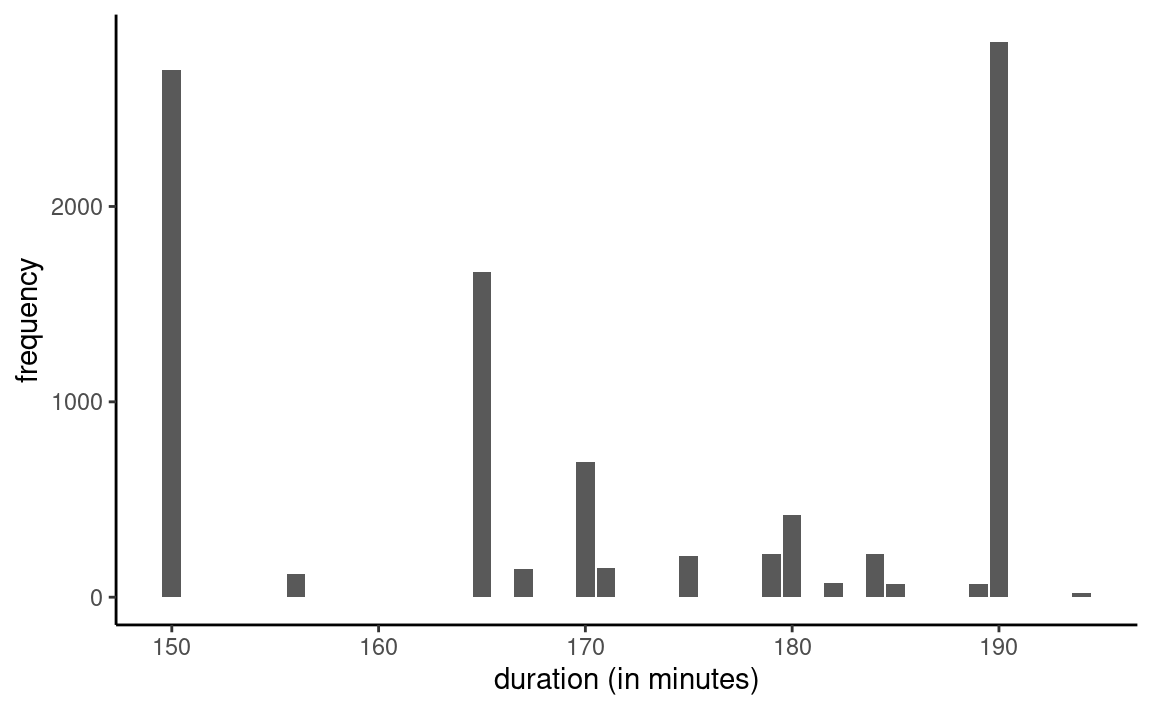
How do we make sense of this result? Let us consider the mean travel time of high speed Spanish trains (AVE) between Madrid and Barcelona that are operated by Renfe.
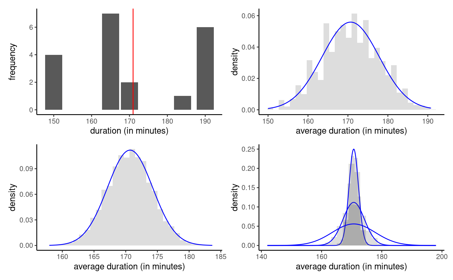
Our exploratory data analysis showed previously that the duration is the one advertised on the ticket: there are only 15 unique travel time. Based on 9603 observations, we estimate the mean travel time to be 170 minutes and 41 seconds. Figure 1.11 shows the empirical distribution of the data.
Consider now samples of size \(n=10\), drawn repeatedly from the population: in the first sample, the sample mean is 169.3 minutes, whereas we get an estimate of 167 minutes in our second , 157.9 minutes in the third, etc.
We draw \(B=1000\) different samples, each of size \(n=5\), from two millions records, and calculate the sample mean in each of them. The top right panel of Figure 1.12 is a histogram of the sample means when \(n=5\), whereas the bottom left panel shows the same thingfor \(n=20.\) The last graph of Figure 1.12 shows the impact of the increase in sample size: whereas the normal approximation is okay-ish for \(n=5\), it is indistinguishable from the normal approximation for \(n=20.\) As \(n\) increases and the sample size gets bigger, the quality of the approximation improves and the curve becomes more concentrated around the true mean. Even if the distribution of the travel time is discrete, the mean is approximately normal.
We considered a single distribution in the example, but you could play with other distributions and vary the sample size to see when the central limit theorem kicks in usng this applet.
The central limit theorem underlies why scaled test statistics which have sample mean zero and sample variance 1 have a standard null distribution in large sample: this is what guarantees the validity of our inference!
Gosset, William Sealy. 1908.
“The Probable Error of a Mean.” Biometrika 6 (1): 1–25.
https://doi.org/10.1093/biomet/6.1.1.