5 Correlated and longitudinal data

Violations of the hypothesis of the linear model impact the validity of statistical inference. Whereas the last chapter followed on generalizations of the linear regression to handle non-normality of the response, we consider now extensions of the linear regression model that account for dependence over time or group heteroscedasticity.

We derived the ordinary least squares estimator using maximum likelihood under the assumption of independent and homoscedastic normal errors. For normally distributed data, the covariance matrix \(\boldsymbol{\Sigma}\) encodes the dependence between observations: off-diagonal elements of the covariance matrix are zero for independent observations, whereas the diagonal elements, which encode the variance, are equal for homoscedastic observations. An alternative way of writing the likelihood of the \(n\) sample is to view the latter as a single realization of an \(n\) dimensional random vector with \(\boldsymbol{Y} \sim \mathsf{No}_n(\mathbf{X}\boldsymbol{\beta}, \sigma^2, \mathbf{I}_n)\). From there, it is easy to see how one can relax the independence and homoscedasticity assumption by writing the covariance matrix \(\boldsymbol{\Sigma}\) in terms of few parameter \(\boldsymbol{\psi}\) and by obtaining the likelihood-based estimators of \(\boldsymbol{\beta}\) and \(\boldsymbol{\psi}\).

5.1 Longitudinal data

The parametrization of the covariance matrix requires some more insight into the dependence structure of the data. Most of the dependence arises from time dependence between consecutive measurements of an observation. This section focuses on longitudinal data, or repeated measurements. These consist of short time series which are collected over different “individuals”: the assumption of independence could hold for measurements of different individuals, but not for measurements of the same individual.

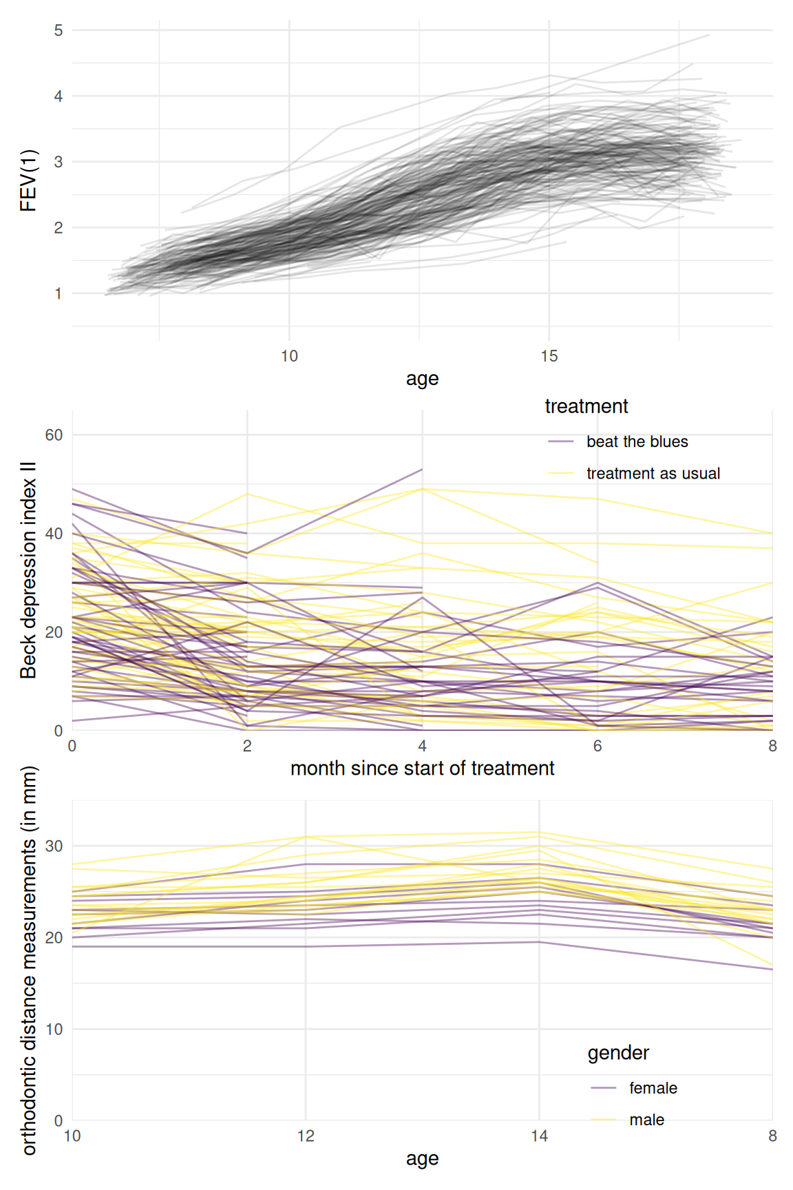
Figure 5.1: Spaghetti plots of longitudinal data: spirometry data from the Six Cities Study of Air Pollution and Health (left), clinical trial data for the ‘Beat the Blues’ cognitive behavioural program (middle) and orthodontic measurements of children (bottom).

We can see from Figure 5.1 that there are a handful of observations per patient and that the overall increase in lung capacity as measured by FEV(1) increases with age. In the fev1 database, the number of observations per individual varies from 1 to 12.

The data we will handled are stored in tables or frames. If the data frame is stocked in long format, each line corresponds to an observation and each column to a variable: the entries of the data base contain the (numeric) values.

The alternative is wide format, whereby the columns represent categorical variables and the entries are values of the response for a specific category (notably contingency tables). Figure 5.2 shows the difference between the two structures. Software typically require long formatted database for modelling purposes.

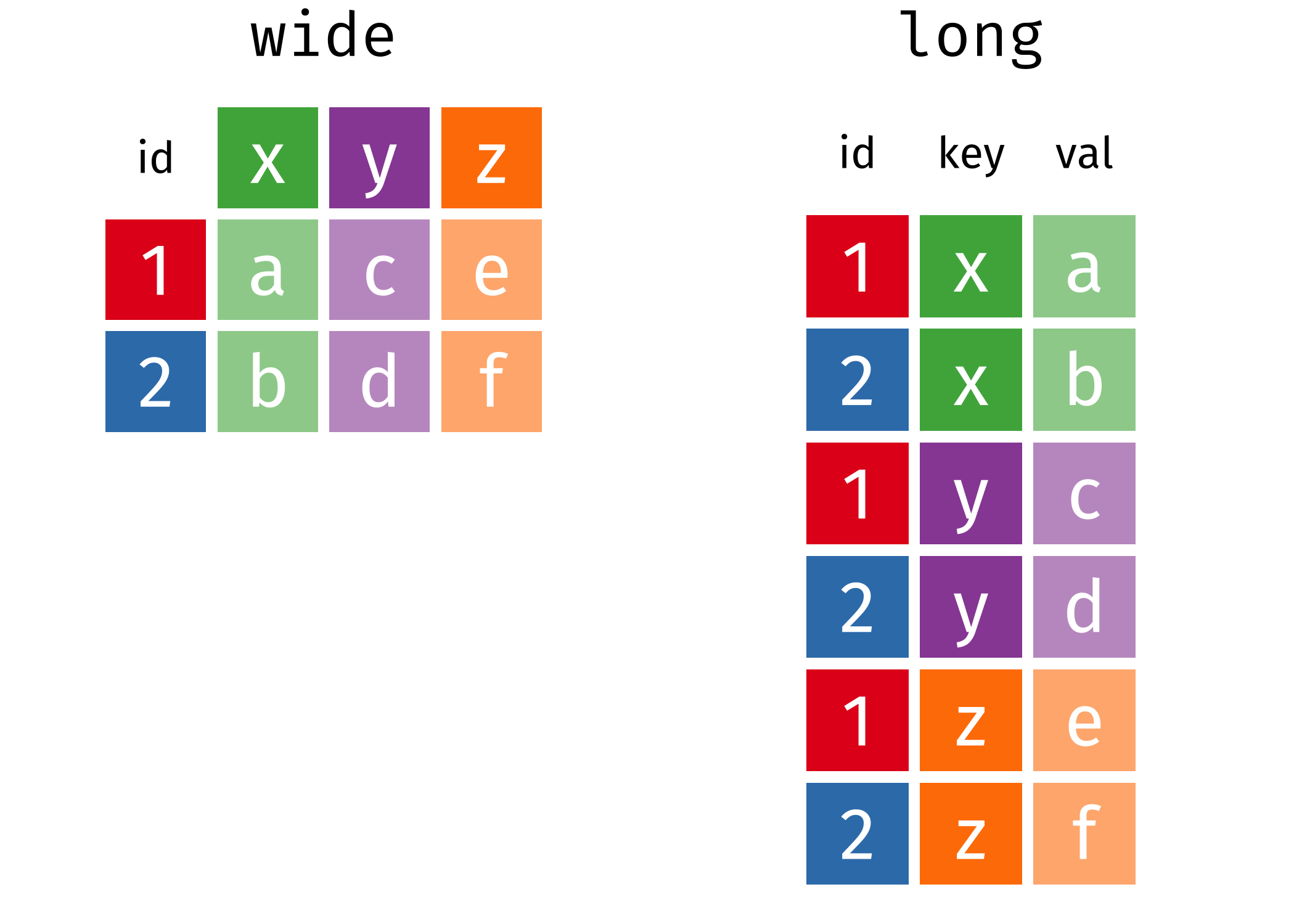
Figure 5.2: Long versus wide-format for data tables (illustration by Garrick Aden-Buie).