2 Linear regression

A linear regression is a model for the conditional mean of a response variable \(Y\) as a function of \(p\) explanatory variables (also termed regressors or covariates), \[\begin{align} \mathsf{E}(Y \mid \mathbf{X})=\beta_0 + \beta_1\mathrm{X}_{1} + \cdots + \beta_p \mathrm{X}_{p}. \tag{2.1} \end{align}\] The mean of \(Y\) is conditional on the values of the observed covariate \(\mathbf{X}\); this amounts to treating them as non-random, known in advance.

In practice, any model is an approximation of reality. An error term is included to take into account the fact that no exact linear relationship links \(\mathbf{X}\) and \(Y\) (otherwise this wouldn’t be a statistical problem), or that measurements of \(Y\) are subject to error. The random error term \(\varepsilon\) will be the source of information for our inference, as it will quantify the goodness of fit of the model.

We can rewrite the linear model in terms of the error for a random sample of size \(n\): denote by \(Y_i\) the value of the response for observation \(i\), and \(\mathrm{X}_{ij}\) the value of of the \(j\)th explanatory variable of observation \(i\). The model is \[\begin{align} Y_i = \beta_0 + \beta_1 \mathrm{X}_{i1} + \ldots + \beta_p \mathrm{X}_{ip} +\varepsilon_{i}, \qquad i =1, \ldots, n, \tag{2.2} \end{align}\] where \(\varepsilon_i\) is the additive error term specific to observation \(i\). While we may avoid making distributional assumption about \(\varepsilon_i\), we nevertheless fix its expectation to zero to encode the fact we do not believe the model is systematically off,, so \(\mathsf{E}(\varepsilon_i \mid \boldsymbol{X}_i)=0\) \((i=1, \ldots, n)\).

One important remark is that the model is linear in the coefficients \(\boldsymbol{\beta}\in \mathbb{R}_{p+1}\), not in the explanatory variables! the latter are arbitrary and could be (nonlinear) functions of other explanatory variables, for example \(\mathrm{X}=\ln(\texttt{years})\), \(\mathrm{X}=\texttt{horsepower}^2\) or \(\mathrm{X}= \mathsf{I}_{\texttt{man}}\cdot\mathsf{I}_{\texttt{full}}\). The mean of the response is specified as a linear combination of explanatory variables. This is at the core of the flexibility of the linear regression, which is used mainly for the following purposes:

1. Evaluate the effects of covariates \(\mathbf{X}\) on the mean response of \(Y\).
2. Quantify the influence of the explanatories \(\mathbf{X}\) on the response and test for their significance.
3. Predict the response for new sets of explanatories \(\mathbf{X}\).

2.1 Introduction

Linear regression is the most famous and the most widely used statistical model around. The name may appear reductive, but many tests statistics (t-tests, ANOVA, Wilcoxon, Kruskal–Wallis) can be formulated using a linear regression, while models as diverse as trees, principal components and deep neural networks are just linear regression model in disguise. What changes under the hood between one fancy model to the next are the optimization method (e.g., ordinary least squares, constrained optimization or stochastic gradient descent) and the choice of variables entering the model (spline basis for nonparametric regression, indicator variable selected via a greedy search for trees, activation functions for neural networks).

This chapter explores the basics of linear regression, parameter interpretation and testing for coefficients and sub-models. Analysis of variance will be presented as special case of linear regression.

To make concepts and theoretical notions more concrete, we will use data from a study performed in a college in the United States. The goal of the administration who collected these information was to investigate potential gender inequality in the salary of faculty members. The data contains the following variables:

• salary: nine-month salary of professors during the 2008–2009 academic year (in thousands USD).
• rank: academic rank of the professor (assistant, associate or full).
• field: categorical variable for the field of expertise of the professor, one of applied or theoretical.
• sex: binary indicator for sex, either man or woman.
• service: number of years of service in the college.
• years: number of years since PhD.

Before drafting a model, a quick look at the data is in due order. If salary increases with year, there is more heterogeneity in the salary of higher ranked professors: logically, assistant professors are either promoted or kicked out after at most 6 years according to the data. The limited number of years prevents large variability for their salaries.

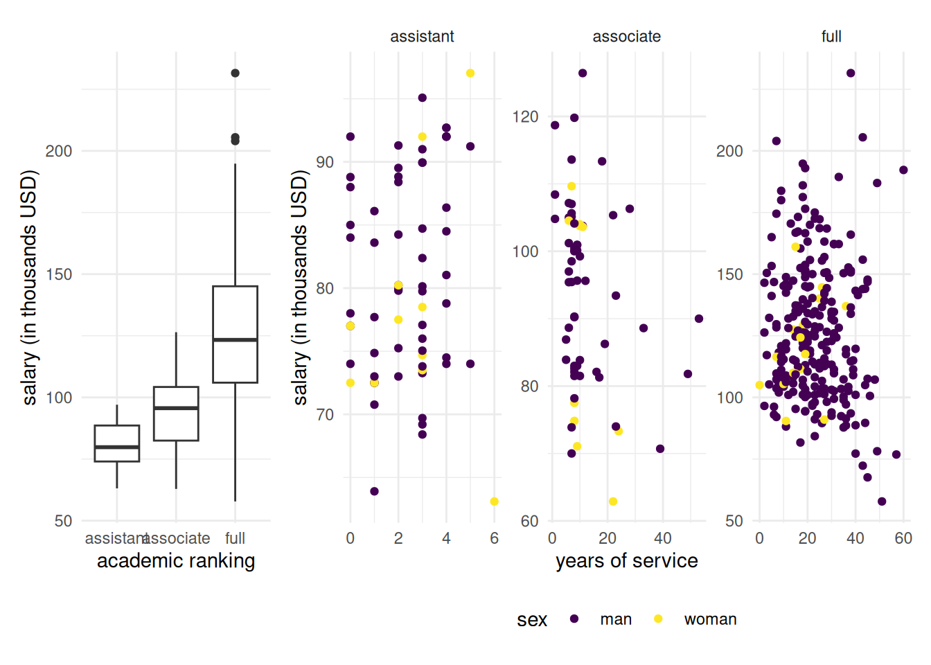
Figure 2.1: Exploratory data analysis of \(\texttt{college}\) data: salaries of professors as a function of the number of years of service and the academic ranking

Salary increases over years of service, but its variability also increases with rank. Note the much smaller number of women in the sample: this will impact our power to detect differences between sex. A contingency table of sex and academic rank can be useful to see if the proportion of women is the same in each rank: women represent 16% of assistant professors and 16% of associate profs, but only 7% of full professors and these are better paid on average.

Table 2.1: Contingency table of the number of prof in the college by sex and academic rank.

	assistant	associate	full
man	56	54	248
woman	11	10	18

The simple linear regression model only includes a single explanatory variable and defines a straight line linking two variables \(\mathrm{X}\) and \(Y\) by means of an equation of the form \(y=a+bx\); Figure 2.2 shows the line passing through the scatterplot for years of service.

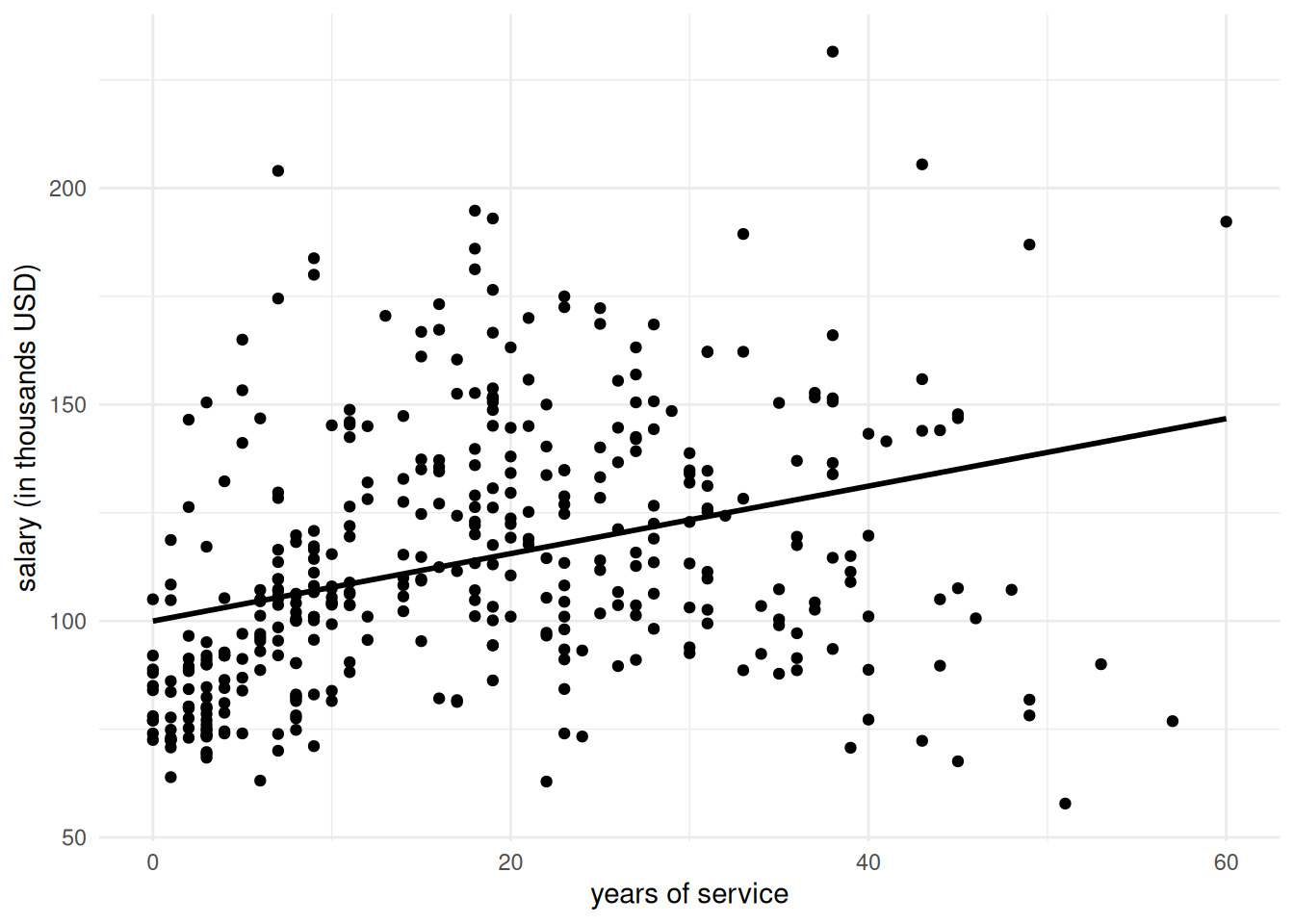
Figure 2.2: Simple linear regression model for the salary of professors as a function of the number of years of service; the line is the solution of the least squares problem.

2.2 Ordinary least squares

The ordinary least square estimators \(\widehat{\boldsymbol{\beta}}=(\widehat{\beta}_0, \ldots, \widehat{\beta}_p)\) are the values that simultaneously minimize the Euclidean distance between the random observations \(Y_i\) and the fitted values \[\begin{align*} \widehat{Y}_i &= \widehat{\beta}_0 + \widehat{\beta}_1 \mathrm{X}_{i1} + \cdots + \widehat{\beta}_p \mathrm{X}_{ip}, \qquad i =1, \ldots, n. \end{align*}\] In other words, the least square estimators are the solution of the convex optimization problem \[\begin{align*} \widehat{\boldsymbol{\beta}} &=\min_{\boldsymbol{\beta} \in \mathbb{R}^{p+1}}\sum_{i=1}^n (Y_i-\widehat{Y}_i)^2= \min_{\boldsymbol{\beta}} \|\boldsymbol{Y}-\mathbf{X}\boldsymbol{\beta}\|^2 \end{align*}\] This system of equations has an explicit solution which is better expressed using matrix notation: this amounts to expressing equation (2.2) with one observation per line.

Consider the matrices \[\begin{align*} \boldsymbol{Y} = \begin{pmatrix} Y_1 \\ Y_2 \\ \vdots \\ Y_n \end{pmatrix} , \; \boldsymbol{\varepsilon} = \begin{pmatrix} \varepsilon_1 \\ \varepsilon_2 \\ \vdots \\ \varepsilon_n \end{pmatrix} , \; \mathbf{X} = \begin{pmatrix} \mathrm{X}_{11} & \mathrm{X}_{12} & \cdots & \mathrm{X}_{1p} \\ \mathrm{X}_{21} & \mathrm{X}_{22} & \cdots & \mathrm{X}_{2p} \\ \vdots & \vdots & \ddots & \vdots \\ \mathrm{X}_{n1} & \mathrm{X}_{n2} & \cdots & \mathrm{X}_{np} \end{pmatrix} , \; \boldsymbol{\beta} = \begin{pmatrix} \beta_1 \\ \beta_2 \\ \vdots \\ \beta_p \end{pmatrix} \end{align*}\] The model in compact form is \[\begin{align*} \boldsymbol{Y} = \mathbf{X} \boldsymbol{\beta} + \boldsymbol{\varepsilon}. \end{align*}\] The ordinary least squares estimator solves the unconstrained optimization problem \[\begin{align*} \widehat{\boldsymbol{\beta}}=\min_{\boldsymbol{\beta} \in \mathbb{R}^{p+1}}(\boldsymbol{y}-\mathbf{X}\boldsymbol{\beta})^\top(\boldsymbol{y}-\mathbf{X}\boldsymbol{\beta}). \end{align*}\] and a proof is provided in the Appendix. If the \(n \times (p+1)\) matrix \(\mathbf{X}\) is full-rank, we obtain a unique solution to the optimization problem, \[\begin{align} \widehat{\boldsymbol{\beta}} = (\mathbf{X}^{\top} \mathbf{X})^{-1} \mathbf{X}^{\top} \boldsymbol{Y}. \tag{2.3} \end{align}\]

What does the solution to the least squares problem represent in two dimensions? The estimator is the one minimizing the sum of squared residuals: the \(i\)th ordinary residual \(e_i = y_i -\widehat{y}_i\) is the vertical distance between a point \(y_i\) and the fitted value \(\widehat{y}_i\) on the line; the blue segments on Figure 2.3 represent the individual vectors of residuals.

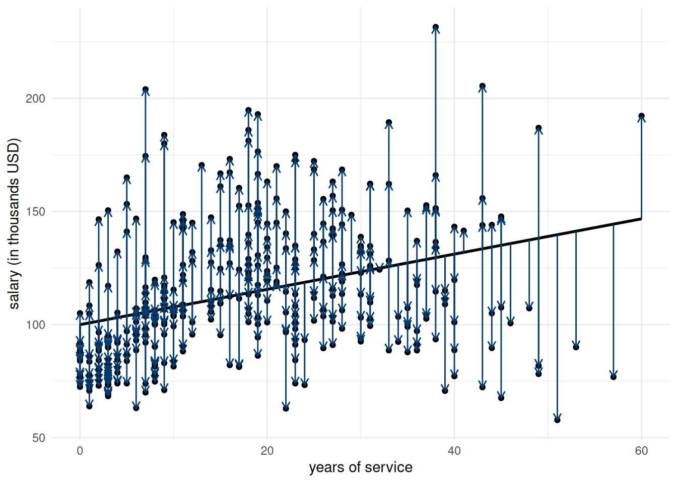
Figure 2.3: Illustration of ordinary residuals added to the regression line (blue vectors).

Remark (Geometry of least squares). If we consider the \(n\) observations as a (column) vector, the term \(\mathbf{X} \widehat{\boldsymbol{\beta}}\) is the projection of the response vector \(\boldsymbol{y}\) on the linear span generated by the columns of \(\mathbf{X}\), \(\mathscr{S}_{\mathbf{X}}\). The ordinary residuals are thus orthogonal to \(\mathscr{S}_{\mathbf{X}}\) and to the fitted values, meaning \(\boldsymbol{e}^\top\widehat{\boldsymbol{y}}=0\). A direct consequence of this fact is that the linear correlation between \(\boldsymbol{e}\) and \(\widehat{\boldsymbol{y}}\) is zero; we will use this property to build graphical diagnostics.

Remark (Complexity of ordinary least squares). This is an aside: in machine learning, you will often encounter linear models fitted using a (stochastic) gradient descent algorithm. Unless your sample size \(n\) or the number of covariates \(p\) is significant (think at the Google scale), an approximate should not be prefered to the exact solution! From a numerical perspective, obtaining the least square estimates requires inverting a \((p+1) \times (p+1)\) matrix \(\mathbf{X}^\top\mathbf{X}\), which is the most costly operation. In general, direct inversion should be avoided because it is not the most numerically stable way of obtaining the solution. R uses the QR decomposition, which has a complexity of \(\mathrm{O}(np^2)\). Another more stable alternative, which has the same complexity but is a bit more costly is use of a singular value decomposition.

Any good software will calculate ordinary least square estimates for you. Keep in mind that there is an explicit and unique solution provided your model matrix \(\mathbf{X}\) doesn’t contain collinear columns. If you have more than one explanatory variable, the fitted values lie on a hyperplan (which is hard to represent graphically). Mastering the language and technical term (fitted values, ordinary residuals, etc.) is necessary for the continuation.

2.3 Interpretation of the model parameters

What do the \(\boldsymbol{\beta}\) parameters of the linear model represent? In the simple case presented in Figure 2.2, the equation of the line is \(\widehat{Y} = \widehat{\beta}_0 + \widehat{\beta}_1\mathrm{X}_1\), \(\beta_0\) is the intercept (the mean value of \(Y\) when \(\mathrm{X}_1=0\)) and \(\beta_1\) is the slope, i.e., the average increase of \(Y\) when \(\mathrm{X}_1\) increases by one unit.

In some cases, the intercept is meaningless because the value \(\mathrm{X}_1=0\) is impossible (e.g., \(\mathrm{X}_1\) represents the height of a human). In the same vein, there may be no observation in a neighborhood of \(\mathrm{X}_1=0\), even if this value is plausible, in which case the intercept is an extrapolation.

If the columns of \(\mathbf{X}\) are arbitrary, it is customary to include an intercept: this amounts to including \(\mathbf{1}_n\) as column of the model matrix \(\mathbf{X}\). Because the residuals are orthogonal to the columns of \(\mathbf{X}\), their mean is zero, since \(n^{-1}\mathbf{1}_n^\top\boldsymbol{e}=\bar{\boldsymbol{e}}=0\). In general, we could also obtain mean zero residuals by including a set of vectors in \(\mathbf{X}\) that span \(\mathbf{1}_n\).

In our example, the equation of the fitted line of Figure 2.2 is \[\widehat{\texttt{salary}} = 99.975 + 0.78\texttt{service}.\] The average salary of a new professor would then be 99974.653 dollars, whereas the average annual increase for each additional year of service is 779.569 dollars.

If the response variable \(Y\) should be continuous (for the least square criterion to be meaningful), we place no such restriction on the explanatories. The case of dummies in particular is common: these variables are encoded using binary indicators (\(0/1\)). Consider for example the sex of the professors in the study: \[\texttt{sex} = \begin{cases} 0 , & \text{for men},\\ 1, & \text{for women.} \end{cases} \] The equation of the simple linear model that includes the binary variable \(\texttt{sex}\) is \(\texttt{salary} = \beta_0 + \beta_1 \texttt{sex} + \varepsilon\). Let \(\mu_0\) denote the average salary of mean and \(\mu_1\) that of women. The intercept \(\beta_0\) can be interpreted as usual: it is the average salary when \(\texttt{sex}=0\), meaning that \(\beta_0=\mu_0\). We can write the equation for the conditional expectation for each sex, \[\begin{align*} \mathsf{E}(\texttt{salary} \mid \texttt{sex})= \begin{cases} \beta_0, & \texttt{sex}=0 \text{ (men)}, \\ \beta_0 + \beta_1 & \texttt{sex}=1 \text{ (women)}. \end{cases} \end{align*}\] A linear model that only contains a binary variable \(\mathrm{X}\) as regressor amounts to specifying a different mean for each of two groups: the average of women is \(\mathsf{E}(\texttt{salary} \mid \texttt{sex}=1) = \beta_0 + \beta_1 = \mu_1\) and \(\beta_1=\mu_1-\mu_0\) represents the difference between the average salary of men and women. The least square estimator \(\widehat{\beta}_0\) is the sample mean of men and \(\widehat{\beta}_1\) is the difference of the sample mean of women and men. The parametrization of the linear model with \(\beta_0\) and \(\beta_1\) is in terms of contrasts and is particularly useful if we want to test for mean difference between the groups, as this amounts to testing \(\mathscr{H}_0: \beta_1=0\). If we wanted our model to directly output the sample means, we would need to replace the model matrix \(\mathbf{X}=[\mathbf{1}_n, \texttt{sex}]\) by \([\mathbf{1}_n- \texttt{sex}, \texttt{sex}]\). The fitted model would be the same because they span the same 2D subspace, but this is not recommended because software treat cases without intercept differently and it can lead to unexpected behaviour (more on this latter).

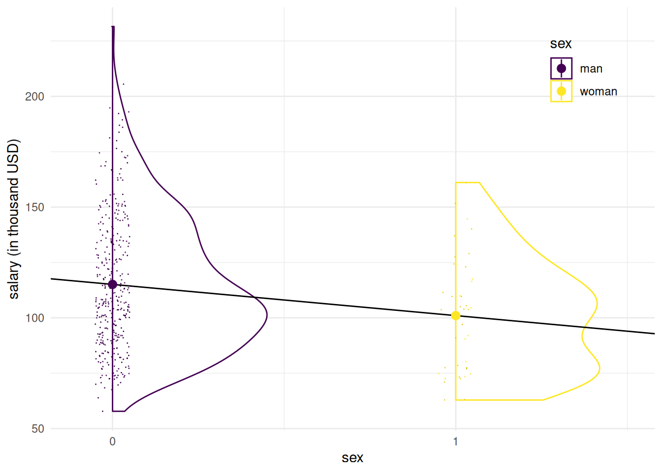
Figure 2.4: Simple linear model for the \(\texttt{college}\) data using the binary variable sex as regressor: even if the equation defines a line, only its values in \(0/1\) are realistic.

If we fit the model with sex only to the college data, we find that the average salary of men is \(\widehat{\beta}_0=1.151\times 10^{5}\) USD and the mean difference estimate of the salary between women and men is \(\widehat{\beta}_1=14088.009\) dollars. Since the estimate is negative, this means women are paid less. Bear in mind that the model is not adequate for determining if there are gender inequalities in the salary distribution: 2.2 shows that the number of years of service and the academic rank strongly impact wages, yet the distribution of men and women is not the same within each rank.

Even if the linear model defines a line, the latter is only meaningful when evaluated at \(0\) or \(1\); Figure 2.4 shows it in addition to sample observations (jittered) and a density estimate for each sex. The colored dot represents the mean, showing that the line does indeed pass through the mean of each group.

A binary indicator is a categorical variable with two levels, so we could extend our reasoning and fit a model with a categorical explanatory variable with \(k\) levels. To do this, we add \(k-1\) indicator variables plus the intercept: if we want to model a different mean for each of the \(k\) groups, it is logical to only include \(k\) parameters in the mean model. We will choose, as we did with sex, a reference category or baseline whose average will be encoded by the intercept \(\beta_0\). The other parameters \(\beta_1, \ldots, \beta_{k-1}\) are contrasts relative to the baseline. The college data includes the ordinal variable rank, which has three levels (assistant, associate and full). We thus need two binary variables, \(\mathrm{X}_1 = \mathsf{I}(\texttt{rank}=\texttt{associate})\) and \(\mathrm{X}_2 = \mathsf{I}(\texttt{rank}=\texttt{full})\); the \(i\)th element of the vector \(\mathrm{X}_1\) is one for an associate professor and zero otherwise. The linear model is \[\begin{align*} \texttt{salary} =\beta_0 + \beta_1 \mathrm{X}_1+\beta_2\mathrm{X}_2 + \varepsilon, \end{align*}\] and the conditional expectation of salary \[\begin{align*} \mathsf{E}(\texttt{salary} \mid \texttt{rank})= \begin{cases} \beta_0, & \texttt{rank}=\texttt{assistant},\\ \beta_0 + \beta_1 & \texttt{rank}=\texttt{associate},\\ \beta_0 + \beta_2 & \texttt{rank}=\texttt{full}, \end{cases} \end{align*}\] Thus \(\beta_1\) (respectively \(\beta_2\)) are the difference between the average salary of associate (respectively full) professors and assistant professors. The choice of the baseline category is arbitrary and all choices yield the same model: only the interpretation changes from one parametrization to the next. For an ordinal variable, it is recommended to choose the smallest or the largest category to ease comparisons.

The models we have fitted so far are not adequate because they ignore variables that are necessarily to correctly explain variations in salaries: Figure 2.1 show for example that rank is critical for explaining the salary variations in the college. We should thus fit a model that include those simultaneously to investigate the gender gap (which consists of differences that are unexplained by other factors). Before doing this, we come back to the interpretation of the parameters in the multiple linear regression setting.

Consider the model \(Y= \beta_0 + \beta_1 \mathrm{X}_1 + \cdots + \beta_p\mathrm{X}_p + \varepsilon\). The intercept \(\beta_0\) represents the mean value of \(Y\) when all of the covariates are set to zero, \[\begin{align*} \beta_0 &= \mathsf{E}(Y \mid \mathrm{X}_1=0,\mathrm{X}_2=0,\ldots,\mathrm{X}_p=0). \end{align*}\] For categorical variables, this yields the baseline, whereas we fix the continous variables to zero: again, this may be nonsensical depending on the study. The coefficient \(\beta_j\) \((j \geq 1)\) can be interpreted as the mean increase of the response \(Y\) when \(\mathrm{X}_j\) increases by one unit, all other things being equal (ceteris paribus); e.g., \[\begin{align*} \beta_1 &= \mathsf{E}(Y \mid \mathrm{X}_1=x_1+1,\mathrm{X}_2=x_2,\ldots,\mathrm{X}_p=x_p) \\ & \qquad \qquad - \mathsf{E}(Y \mid \mathrm{X}_1=x_1,\mathrm{X}_2=x_2,\ldots,\mathrm{X}_p=x_p) \\ &= \left\{\beta_0 + \beta_1 (x_1+1) + \beta_2 x_2 + \cdots +\beta_p \mathrm{X}_p \right\} \\ & \qquad \qquad -\left\{\beta_0 + \beta_1 x_1 + \beta_2 x_2 + \cdots +\beta_p \mathrm{X}_p \right\} \end{align*}\] It is not always possible to fix the value of an explanatory if multiple columns of \(\mathbf{X}\) contains functions/transformations of it. For example, if we included a polynomial of order \(k\) for some variable \(\mathrm{X}\), \[\begin{align*} Y=\beta_0+ \beta_1 \mathrm{X}+ \beta_2 \mathrm{X}^2 + \ldots +\beta_k \mathrm{X}^k + \varepsilon. \end{align*}\] If we include a term of order \(k\), \(\mathrm{X}^k\), we must always include the lower order terms \(1, \mathrm{X}, \ldots, \mathrm{X}^{k-1}\) to make sure the resulting model is interpretable (otherwise, it amounts to a particular class of polynomials with some zero coefficients). Interpreting nonlinear effects (even polynomials, for which \(k\leq 3\) in practice), is complicated because the effect of an increase of one unit of \(\mathrm{X}\) depends of the value of the latter.

Example 2.1 (Auto data) We consider a linear regression model for the fuel autonomy of cars as a function of the power of their motor (measured in horsepower) from the auto dataset. The postulated model, \[ \texttt{mpg}_i = \beta_0 + \beta_1 \texttt{horsepower}_i + \beta_2 \texttt{horsepower}_i^2 + \varepsilon_i, \] includes a quadratic term. Figure 2.5 shows the scatterplot with the fitted regression line, above which the line for the simple linear regression for horsepower is added.

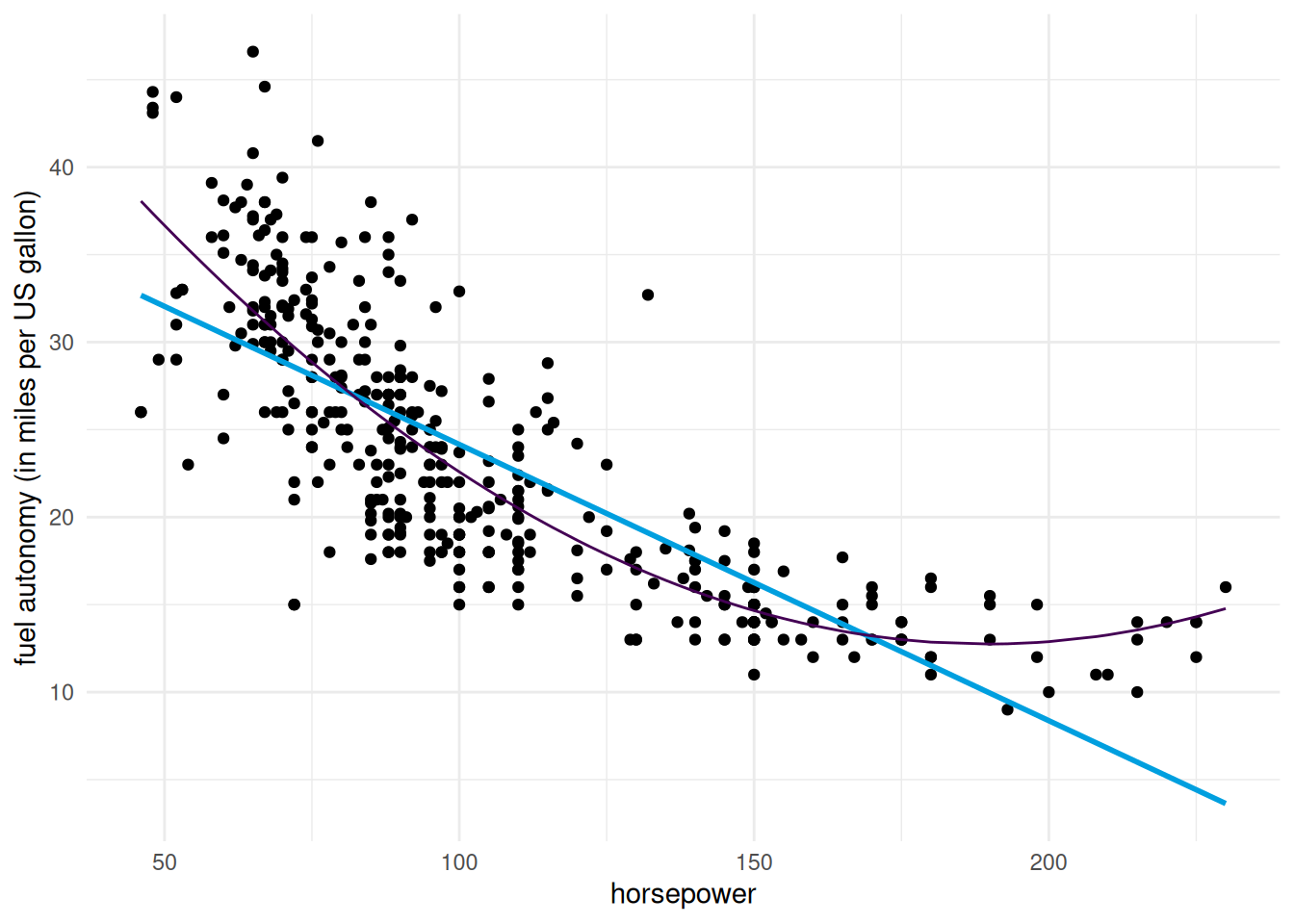
Figure 2.5: Linear regression models for the fuel autonomy of cars as a function of motor power

It appears graphically that the quadratic model fits better than the simple linear alternative: we will assess this hypothesis formally later. For the degree two polynomial, Figure 2.5 show that fuel autonomy decreases rapidly when power increases between 50 to 100, then more slow until 189.35 hp. After that, the model postulates that autonomy increases again as evidenced by the scatterplot, but beware of extrapolating (weird things can happen beyond the range of the data, as exemplified by Hassett’s cubic model for the number of daily cases of Covid19 in the USA).

The representation in Figure 2.5 may seem counter-intuitive given that we fit a linear model, but it is a 2D projection of 3D coordinates for the equation \(\beta_0 + \beta_1x-y +\beta_2z =0\), where \(x=\texttt{horsepower}\), \(z=\texttt{horsepower}^2\) and \(y=\texttt{mpg}\). Physics and common sense force \(z = x^2\), and so the fitted values lie on a curve in a 2D subspace of the fitted plan, as shown in grey in the 3D Figure 2.6.

Figure 2.6: 3D graphical representation of the linear regression model for the \(\texttt{auto}\) data.

Remark (There are better alternatives to polynomials for modelling nonlinear effects). Generally speaking, one uses flexible basis vectors (splines) rather than polynomials for smoothing when the relation between the response \(Y\) and an explanatory variable \(\mathrm{X}\) is nonlinear; one then adds a penalty term to prevent overfitting and control the wiggliness. A better (physical) understanding of the system, or a theoretical model can also guide the choice of functional form to use.

The coefficient \(\beta_j\) in Eq. (2.1) represents the marginal contribution of \(\mathrm{X}_j\) when all the other covariates are included in the model and which is not explained by them. This can be represented graphically by projecting \(Y\) and \(\mathrm{X}_j\) in the orthogonal complement of \(\mathbf{X}_{-j}\) (the matrix containing all but the \(j\)th column \(\mathrm{X}_j\)). The added-variable plot is a graphical tool showing this projection: the residuals from the linear regression of \(Y\) onto \(\mathscr{S}(\mathbf{X}_{-j})\) are mapped to the \(y\)-axis, whereas the residuals from the linear regression of \(\mathrm{X}_j\) as a function of \(\mathbf{X}_{-j}\) are shown on the \(x\)-axis. The regression line passes through (\(0,0\)) and its slope is \(\widehat{\beta}_j\). This graphical diagnostic is useful for detecting collinearity and the impact of outliers.

Example 2.2 (Wage inequality in an American college) We consider a multiple regression model for the college data that includes sex, academic rank, field of study and the number of years of service as regressors.

If we multiply \(\texttt{salary}\) by a thousand to get the resulting estimates in US dollars, the postulated model is \[\begin{align*} \texttt{salary}\times 1000 &= \beta_0 + \beta_1 \texttt{sex}_{\texttt{woman}} +\beta_2 \texttt{field}_{\texttt{theoretical}} \\&\quad +\beta_3 \texttt{rank}_{\texttt{associate}} +\beta_4 \texttt{rank}_{\texttt{full}} +\beta_5 \texttt{service} + \varepsilon. \end{align*}\]

Table 2.2: Estimated coefficients of the linear model for the \(\texttt{college}\) (in USD, rounded to the nearest dollar).

\(\widehat{\beta}_0\)	\(\widehat{\beta}_1\)	\(\widehat{\beta}_2\)	\(\widehat{\beta}_3\)	\(\widehat{\beta}_4\)	\(\widehat{\beta}_5\)
86596	-4771	-13473	14560	49160	-89

The interpretation of the coefficients is as follows:

• The estimated intercept is \(\widehat{\beta}_0=86596\) dollars; it corresponds to the mean salary of men assistant professors who just started the job and works in an applied domain.
• everything else being equal (same field, academic rank, and number of years of service), the estimated salary difference between a woman and is estimated at \(\widehat{\beta}_1=-4771\) dollars.
• ceteris paribus, the salary difference between a professor working in a theoretical field and one working in an applied field is \(\beta_2\) dollars: our estimate of this difference is \(-13473\) dollars, meaning applied pays more than theoretical.
• ceteris paribus, the estimated mean salary difference between associate and assistant professors is \(\widehat{\beta}_3=14560\) dollars.
• ceteris paribus, the estimated mean salary difference between full and assistant professors is \(\widehat{\beta}_4=49160\) dollars.
• au sein d’un même échelon, chaque année supplémentaire de service mène à une augmentation de salary annuelle moyenne de \(\widehat{\beta}_5=-89\) dollars.

All other factors taken into account, women get paid less than men. It remains to see if this difference is statistically significant. Perhaps more surprising, the model estimates that salary decreases with every additional year of service: this seems counterintuitive when looking at Figure 2.2, which showed a steady increas of salary over the years. However, this graphical representation is misleading because Figure 2.1 showed that academic ranking mattered the most. Once all the other factors are accounted for, years of service serves to explain the salary of full professors who have been working unusual amounts of time and who gain less than the average full professor, as shown by the added-variable plot of Figure 2.7.

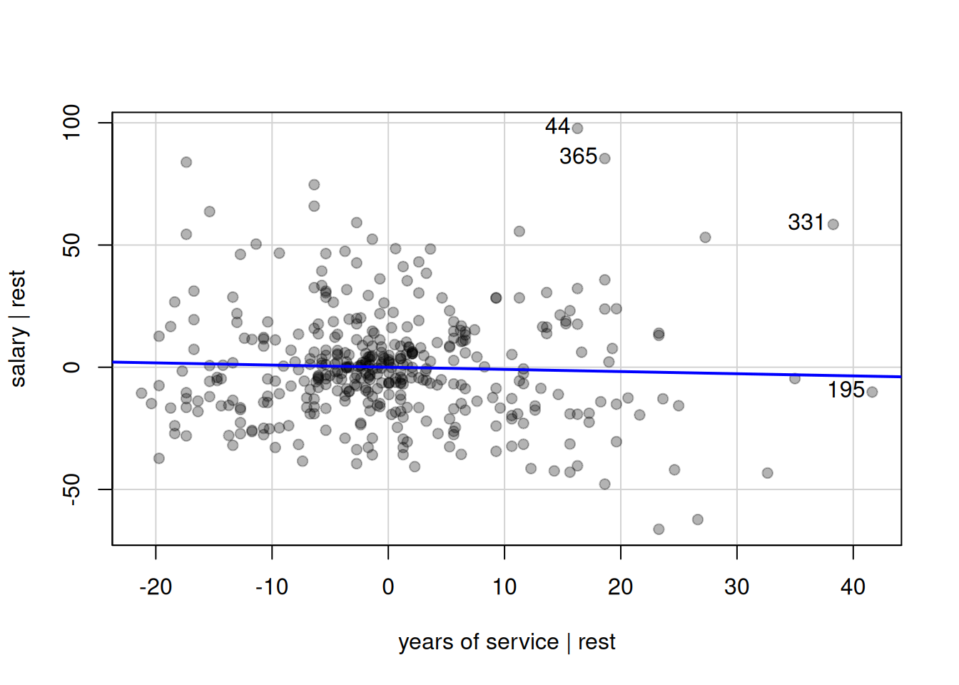
Figure 2.7: Added-variable plot for years of service in the linear regression model of the \(\texttt{college}\) data.

Details about implementation of linear models using R are provided in the Appendix.

2.4 Tests for parameters of the linear model

We need to make further assumptions in order to carry out inference and build testing procedures for the mean model parameters of the linear model. In order to get a tractable distribution for test statistics, it is customary to assume that the disturbances \(\boldsymbol{\varepsilon}\) are independent normal random variables with mean zero and common variance \(\sigma^2\). It follows that \(Y_1, \ldots, Y_n\) are conditionally independent random variables with \[\begin{align*} \mathsf{E}(Y_i \mid \mathbf{X}_i)=\beta_0 + \sum_{j=1}^p \mathrm{X}_{ij}\beta_j, \quad \mathsf{Va}(Y_i\mid \mathbf{X}_i)= \sigma^2, \quad i=1, \ldots, n. \end{align*}\] Under this hypothesis, the least square estimators for the mean parameters coincide with the maximum likelihood estimators. The advantage of imposing this (more stringent than necessary) assumption is that we can use our toolbox for testing. The theory underlying likelihood tests is presented in the chapter on likelihood-based inference. Assuming normal errors leads to exact distributions for the test statistics (which also coincide with the asymptotic ones in large samples).

Of particular interest are tests of restrictions for components of \(\boldsymbol{\beta}\). The large sample properties of the maximum likelihood estimator imply that \[\begin{align*} \widehat{\boldsymbol{\beta}} \stackrel{\cdot}{\sim}\mathsf{No}_{p+1}\left\{\boldsymbol{\beta}, \sigma^2(\mathbf{X}^\top\mathbf{X})^{-1}\right\} \end{align*}\] for sufficiently large sample size. One can thus easily estimate the standard errors from the matrix upon replacing \(\sigma^2\) by an estimator, typically the unbiased estimator of the variance.

In an inferential setting, it’s often important to test whether the effect of an explanatory variable is significant: if \(\mathrm{X}_j\) is binary or continuous, the test for \(\mathscr{H}_0: \beta_j=0\) corresponds to a null marginal effect for \(\mathrm{X}_j\). The null model is a linear regression in which we remove the \((j+1)\)st column of \(\mathbf{X}\), so both models are nested. The Wald test statistic is reported by most software \(W=\widehat{\beta}_j/\mathsf{se}(\widehat{\beta}_j)\) and the null distribution is Student-t with \(n-p-1\) degrees of freedom, which explains the terminology (\(t\) values). In addition to coefficient estimates, it is possible to obtain confidence intervals for \(\beta_j\), which are the usual \(\widehat{\beta}_j \pm t_{n-p-1,\alpha/2} \mathsf{se}(\widehat{\beta}_j)\), with \(t_{n-p-1,\alpha/2}\) denoting the \(1-\alpha/2\) quantile of the \(\mathsf{St}_{n-p-1}\) distribution.

For categorical variables with more than two levels, testing if \(\beta_j=0\) is typically not of interest because the contrast represent the different between the category \(\mathrm{X}_j\) and the baseline: these two categories could have a small difference, but the categorical variable as a whole may still be a useful predictor given the other explanatories. The hypothesis of zero contrast is awkward because it implies a null model in which selected categories are merged.

2.4.1 F-tests for comparison of nested linear models

Consider the full linear model which contains \(p\) predictors, \[\begin{align*} \mathbb{M}_1: Y=\beta_0+\beta_1 \mathrm{X}_1 + \cdots + \beta_g \mathrm{X}_g + \beta_{k+1}\mathrm{X}_{k+1} + \ldots + \beta_p \mathrm{X}_p + \varepsilon. \end{align*}\] Suppose without loss of generality that we want to test \(\mathscr{H}_0: \beta_{k+1}=\beta_{k+2}=\ldots=\beta_p=0\) (one could permute columns of the model matrix to achieve this configuration). The global hypothesis specifies that \((p-k)\) of the \(\beta\) parameters are zero. The restricted model corresponding to the null hypothesis contains only the covariates for which \(\beta_j \neq 0\), \[\begin{align*} \mathbb{M}_0: Y=\beta_0+\beta_1 \mathrm{X}_1 + \ldots + \beta_k \mathrm{X}_k + \varepsilon. \end{align*}\] Let \(\mathsf{SS}_e(\mathbb{M}_1)\) be the residuals sum of squares for model \(\mathbb{M}_1\), \[\begin{align*} \mathsf{SS}_e(\mathbb{M}_1)=\sum_{i=1}^n (Y_i-\widehat{Y}_i^{\mathbb{M}_1})^2, \end{align*}\] where \(\widehat{Y}_i^{\mathbb{M}_1}\) is the \(i\)th fitted value from \(\mathbb{M}_1\). Similarly define \(\mathsf{SS}_e(\mathbb{M}_0)\) for the residuals sum of square of \(\mathbb{M}_0\). Clearly, \(\mathsf{SS}_e(\mathbb{M}_0) \geq \mathsf{SS}_e(\mathbb{M}_1)\) (why?)

The \(F\)-test statistic is \[\begin{align*} F=\frac{\{\mathsf{SS}_e(\mathbb{M}_0)-\mathsf{SS}_e(\mathbb{M}_1)\}/(p-k)}{\mathsf{SS}_e(\mathbb{M}_1)/(n-p-1)} \end{align*}\] Under \(\mathscr{H}_0\), the \(F\) statistic follows a Fisher distribution with \((p-k)\) and \((n-p-1)\) degrees of freedom, \(\mathsf{F}(p-k, n-p-1)\) — \(p-k\) is the number of restrictions, \(n-p-1\) is sample size minus the number of \(\beta\)’s in \(\mathbb{M}_1\).

It turns out that both \(F\) and \(t\)-statistics are equivalent for testing a single coefficient \(\beta_j\): the \(F\)-statistic is the square of the Wald statistic and they lead to the same inference — the \(p\)-value for the test are identical. While it may get reported in tables, the test for \(\beta_0=0\) is not of interest; we keep the intercept merely to centre the residuals.

For normal linear regression, the likelihood ratio test for comparing models \(\mathbb{M}_1\) and \(\mathbb{M}_0\) is a function of the sum of squared residuals: the usual formula simplifies to \(R = n\ln\{\mathsf{SS}_e(\mathbb{M}_0)/\mathsf{SS}_e(\mathbb{M}_1)\}\). This is reminiscent of the \(F\)-statistic formula and the two are in fact intimately related modulo null distribution and scaling. The \(t\)-tests and \(F\)-tests presented above could thus both be viewed as particular cases of likelihood-based tests.

Consider the college data example and the associated linear model with rank, sex, years of service and field as covariates.

Table 2.3: Table of linear regression coefficients with associated standard errors, Wald tests and \(p\)-values based on Student-\(t\) distribution

term	estimate	std. error	Wald stat.	p-value
(Intercept)	86.596	2.96	29.25	< 0.001
sex [woman]	-4.771	3.878	-1.23	0.22
field [theoretical]	-13.473	2.315	-5.82	< 0.001
rank [associate]	14.56	4.098	3.55	< 0.001
rank [full]	49.16	3.834	12.82	< 0.001
service	-0.089	0.112	-0.8	0.43

Table 2.3 shows the estimated coefficients (in thousands of dollars). The coefficients are the least squares estimates \(\widehat{\boldsymbol{\beta}}\), the standard errors are the square root of the diagonal elements of \(S^2(\mathbf{X}^\top\mathbf{X})^{-1}\). The Wald (or t-) statistic is simply \(W=\widehat{\beta}/\mathsf{se}(\widehat{\beta})\) for \(\mathscr{H}_0: \beta_j=0\): given two of the three estimates, we could easily recover the third using the formula for the test. The \(p\)-values are for the two-sided alternative test with \(\mathscr{H}_a: \beta_j \neq 0\).

The interpretation is usual: \(p\)-values that are less than our prescribed level \(\alpha\) do not contribute significantly given the other variables already in the model. Neither years of service nor sex are statistically different from zero given all the other variables. The test for \(\beta_{\texttt{sex}}\) is comparing the model with all covariates (including service), and vice-versa. Note that the conclusion changes depending on the model: both coefficients would be statistically significant had we removed rank from the set of covariates, because they are correlated. The gender imbalance among ranks explains most of the gap between sex, whereas year of service is largely redundant once we account for the jumps due to change of academic rank.

Table 2.4: Type 3 sum of square decomposition table: sum of square decomposition comparing nested models with and without covariates, \(F\)-statistic and associated \(p\)-value.

variable	sum of square	df	F stat.	p-value
(Intercept)	439059.2	1	855.71	< 0.001
sex	776.7	1	1.51	0.22
field	17372.5	1	33.86	< 0.001
rank	102883.1	2	100.26	< 0.001
service	324.5	1	0.63	0.43
Residuals	200620.4	391

Table 2.4 gives the \(F\)-statistics values and the associated \(p\)-values. The sum of squares represent the difference \(\mathsf{SS}_e(\mathbb{M}_0)-\mathsf{SS}_e(\mathbb{M}_1)\) for various null models \(\mathbb{M}_0\), except the last line for residuals which reports \(\mathsf{SS}_e(\mathbb{M}_1)\). You can verify that (up to rounding) these \(p\)-pvalues are identical to those of the Wald test in the output when df=1. The only categorical variable here with more than one level is rank, and it is strongly significant: removing it from the model leads to a sharp decrease in fit.

We could have also easily computed the likelihood ratio test to compare the models: for example, the log likelihood for the full model is -1799.027 and that of the model without rank is -1881.202, so the likelihood ratio statistic would be 164.349 and this is strongly significant when compared to the \(\chi^2_2\) distribution (both likelihood ratio test and \(F\)-test give a \(p\)-value of \(2.2 \times 10^{-16}\)).

2.5 Coefficient of determination

When we specify a model, the error term \(\boldsymbol{\varepsilon}\) accounts for the fact no perfect linear relationship characterizes the data (if it did, we wouldn’t need statistic to begin with). Once we have fitted a model, we estimate the variance \(\sigma^2\); one may then wonder which share of the total variance in the sample is explained by the model.

The total sum of squares, defined as the sum of squared residuals from the intercept-only model, serves as comparison — the simplest model we could come up with would involving every observation by the sample mean of the response and so this gives (up to scale) the variance of the response, \(\mathsf{SS}_c = \sum_{i=1}^n (y_i - \overline{y})^2\). We can then compare the variance of the original data with that of the residuals from the model with covariate matrix \(\mathbf{X}\), defined as \(\mathsf{SS}_e =\sum_{i=1}^n e_i^2\) with \(e_i = y_i - \widehat{\beta}_0 - \sum_{j=1}^p \widehat{\beta}_j\mathrm{X}_j\). We define the coefficient of determination, or squared multiple correlation coefficient of the model, \(R^2\), as \[\begin{align*} R^2 = 1- \frac{\mathsf{SS}_e}{\mathsf{SS}_c} = \frac{\sum_{i=1}^n (y_i - \overline{y})^2- \sum_{i=1}^n e_i^2}{\sum_{i=1}^n (y_i - \overline{y})^2}. \end{align*}\] The coefficient of determination can be interpreted as the square of Pearson’s linear correlation between the response \(\boldsymbol{y}\) and the fitted values \(\widehat{\boldsymbol{y}}\); see the Appendix for a derivation of this fact.

Its important to note that \(R^2\) is not a goodness-of-fit criterion: some phenomena are inherently noisy and even a good model will fail to account for much of the response’s variability. Moreover, one can inflate the value of \(R^2\) by including more explanatory variables: the coefficient is non-decreasing in the dimension of \(\mathbf{X}\), so a model with \(p+1\) covariate will necessarily have a higher \(R^2\) values than only \(p\) of the explanatories. For model comparisons, it is better to employ information criteria, or else rely on the predictive performance if this is the purpose of the regression. Lastly, a model with a high \(R^2\) may imply high correlation, but the relation may be spurious: linear regression does not yield causal models!

2.6 Predictions

When we compute least square estimates, we obtain fitted values \(\widehat{\boldsymbol{y}}\) as \(\mathbf{X}\widehat{\boldsymbol{\beta}}\), where \(\mathbf{X}\) denotes the \(n \times (p+1)\) matrix of original observations. Recalling that \(\mathsf{E}(Y_i \mid \mathbf{X}_i) = \beta_0 + \sum_{j=1}^p \beta_j \mathrm{X}_{ij}\), we can obtain an estimate of the mean surface for any value of \(\mathbf{x}_{n+1} \in \mathbb{R}^p\) by replacing the unknown coefficients \(\boldsymbol{\beta}\) by our estimates \(\widehat{\boldsymbol{\beta}}\) – this actually yields the best linear unbiased predictor of the mean.

If we want to predict the value of a new observation, say \(Y_{n+1}\), with explanatories \(\mathbf{x}_{n+1} = (1, x_1, \ldots, x_p)\), the prediction of the value will also be \(\widehat{y}_{n+1} = \mathbf{x}_{n+1}\widehat{\boldsymbol{\beta}}\) because \[\begin{align*} \mathsf{E}(Y_{n+1} \mid \mathbf{x}_{n+1}) = \mathbf{x}_{n+1}\boldsymbol{\beta} + \mathsf{E}(\varepsilon_{n+1} \mid \mathbf{x}_{n+1}) = \mathbf{x}_{n+1}\boldsymbol{\beta}. \end{align*}\] However, individual observations vary more than averages (which are themselves based on multiple observations). Intuitively, this is due to the added uncertainty of the error term \(\varepsilon_{n+1}\) appearing in the model equation: the variability of new predictions is the sum of uncertainty due to the estimators (based on random data) and the intrinsic variance of the observations assuming the new observation is independent of those used to estimate the coefficients, \[\begin{align*} \mathsf{Va}(Y_{n+1} \mid \mathbf{x}_n) &= \mathsf{Va}(\mathrm{x}_{n+1}\widehat{\boldsymbol{\beta}} + \varepsilon_{n+1} \mid \mathbf{x}_n) \\&=\mathsf{Va}(\mathrm{x}_{n+1}\widehat{\boldsymbol{\beta}} \mid \mathbf{x}_n) +\mathsf{Va}(\varepsilon_{n+1} \mid \mathbf{x}_n) \\& = \sigma^2\mathrm{x}_{n+1}(\mathbf{X}^\top\mathbf{X})^{-1}\mathrm{x}_{n+1}^\top + \sigma^2, \end{align*}\] where \(S^2\) is the unbiased estimator of the variance \(\sigma^2\). The distribution of \(Y_{n+1}\) is by assumption normal, but since we do not know the variance, we base the prediction interval on the Student distribution, viz. \[\begin{align*} \frac{\mathrm{x}_{n+1}\widehat{\boldsymbol{\beta}}-Y_{n+1}}{\sqrt{S^2\{1+\mathrm{x}_{n+1}(\mathbf{X}^\top\mathbf{X})^{-1}\mathrm{x}_{n+1}^\top\}}}\sim \mathsf{St}_{n-p-1}. \end{align*}\] and obtain \(1-\alpha\) prediction interval for \(Y_{n+1}\) by inverting the test statistic, \[\begin{align*} \mathrm{x}_{n+1}\widehat{\boldsymbol{\beta}}\pm \mathfrak{t}_{n-p-1}(\alpha/2)\sqrt{S^2\{1+\mathrm{x}_{n+1}(\mathbf{X}^\top\mathbf{X})^{-1}\mathrm{x}_{n+1}^\top\}}. \end{align*}\] Similar calculations yield the formula for confidence intervals for the mean, \[\begin{align*} \mathrm{x}_{n+1}\widehat{\boldsymbol{\beta}}\pm \mathfrak{t}_{n-p-1}(\alpha/2)\sqrt{S^2\mathrm{x}_{n+1}(\mathbf{X}^\top\mathbf{X})^{-1}\mathrm{x}_{n+1}^\top}. \end{align*}\] The two differ only because of the additional variance of individual observations.

Figure 2.8 shows pointwise uncertainty bands for a simple linear regression of the intention data as a function of fixation, illustrating the limitations of the linear model in this example: the model is not accounting for the fact that our response arises from a bounded discrete distribution with integer values ranging from 2 to 14. The middle line gives the prediction of individuals as we vary their fixation time. Looking at the formula for the confidence, it is clear that the bands are not linear (we consider the square root of a function that involves the predictors), but it is not obvious that the uncertainty increases as you move away from the average of the predictors. This is more easily seen by replicating the potential curves that could have happened with different data: I generated new potential slopes from the asymptotic normal distribution of \(\widehat{\boldsymbol{\beta}}\) estimators to show the hyperbolic shape is not surprising: we are basically tilting curves from the average fixation/intention, and they have higher potential from deviating far from the range of observations.

Figure 2.8: Prediction for the simple linear regression of buying intention as a function of fixation time. The plot shows predictions along with pointwise 95% confidence intervals of the mean and the individual predictions.

2.7 Interactions

In the interpretation of the linear model, the effect of an explanatory variable is assumed to be the same, regardless of the other explanatory variables (ceteris paribus). To isolate the effect of \(\beta_j\), we indeed fix the value of the other explanatories and increase by one the variable \(\mathrm{X}_j\) (whenever this makes sense) to obtain the slope coefficient. However, the effect of a covariate may sometimes depend on another explanatory.

A good example of interaction is provided by the insurance dataset. An exploratory data analysis suggested that premiums depended on age, smoker status and body mass index, but through obesity status. It can be best represented graphically by looking at body mass index.

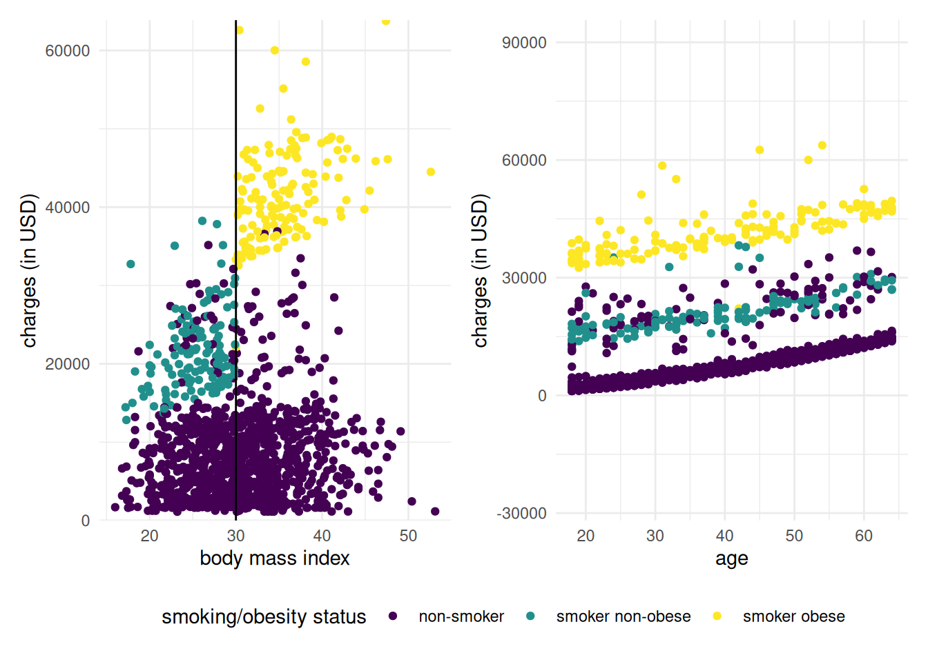
Figure 2.9: Graph of insurance charges against body mass index. The figure clearly shows the interaction: the premium vary for smokers depending on whether or not they are obese, but we see no such behaviour for non-smokers. There is a clear linear increase of charges with age, but it is not clear whether the annual increase is the same for the three groups.

From there, we could create an indicator variable \(\texttt{obese}=\mathsf{I}(\texttt{bmi} \geq 30)\) and add an interaction term between smoker/obese (categorical) and age (continuous) in our mean model. We take non-smoker as baseline category. To make interpretation more meaningful, we rescale age so that \(\texttt{age}=0\) corresponds to 18 years old.

Table 2.5: Table of regression coefficients for the insurance data with interaction terms between age, obesity and smoker status.

term	estimate	std. error	Wald stat.	p-value
(Intercept)	2668.7	362.7	7.36	< 0.001
age	265.9	15	17.7	< 0.001
obesity [obese]	115.3	510.3	0.23	0.82
smoker [yes]	13526.2	803.1	16.84	< 0.001
age * obesity [obese]	1.4	20.1	0.07	0.94
age * smoker [yes]	-5.3	33.5	-0.16	0.87
obesity [obese] * smoker [yes]	19308.7	1110.5	17.39	< 0.001
age * obesity [obese] * smoker [yes]	19.1	44.8	0.43	0.67

The linear regression model has eight parameters, which could be mapped to four intercepts and four different slopes for age; however, the model is parametrized in terms of contrasts, which facilitates testing restrictions.

\[\begin{align*} \texttt{charges} &= \beta_{0} + \beta_{1}\texttt{age} + \beta_{2}\texttt{obese} + \beta_{3}\texttt{smoker} + \beta_{4}\texttt{age} \cdot \texttt{obese} \\&\quad + \beta_{5}\texttt{age} \cdot \texttt{smoker} + \beta_{6}\texttt{obese} \cdot \texttt{smoker} + \beta_{7}\texttt{age} \cdot \texttt{obese} \cdot \texttt{smoker} + \varepsilon \end{align*}\]

Because of the three-way interaction, it is not possible to recover individual parameters by changing the value of the corresponding covariate and keeping everything else constant: changing the smoker status likely impacts multiple regressors simultaneously. To retrieve the interpretation of the different coefficients, we will need to change one parameter at the time, write the mean equation and then isolate the coefficients. Throughout, \(\texttt{obese}\) is a dummy variable equal to one if the person has a body mass index greater than 30 and likewise \(\texttt{smoker}\) if the person is a smoker.

\[\begin{align*} \texttt{charges} = \begin{cases} \beta_{0} + \beta_{1}\texttt{age} & (\mathrm{g}_1)\, \texttt{non-obese}, \texttt{non-smoker} \\ (\beta_{0} + \beta_{2}) + (\beta_{1} + \beta_{4})\texttt{age}, & (\mathrm{g}_2)\, \texttt{obese}, \texttt{non-smoker} \\ (\beta_{0} + \beta_{3}) + (\beta_{1} + \beta_{5})\texttt{age}, & (\mathrm{g}_3)\, \texttt{non-obese}, \texttt{smoker} \\ (\beta_{0} + \beta_{2} + \beta_{3}+ \beta_{6}) + (\beta_{1} + \beta_{4} +\beta_{5} + \beta_7)\texttt{age}, & (\mathrm{g}_4)\, \texttt{obese}, \texttt{smoker} \end{cases} \end{align*}\]

• The intercept \(\beta_0\) is the average at 18 years old of non-smokers who are not obese.
• The slope \(\beta_1\) is the average annual increase in charges for non-smokers who are not obese.
• The parameter \(\beta_2\) is a contrast, the difference between the average charges of 18 years old non-smokers who are obese and those who are not.
• The parameter \(\beta_3\) is a contrast, the difference between the average premium for non-obese 18 years old who smoke and those who don’t.
• The parameter \(\beta_4\) is a contrast, the difference in average annual increase for non-smokers between obese and non-obese adults.
• The parameter \(\beta_5\) is a contrast, the difference in average annual increase for non-obese between smoker and non-smoker adults.

The other two coefficients, \(\beta_6\) and \(\beta_7\) represent differences of average between groups \(\mathrm{g}_1 + \mathrm{g}_4 - \mathrm{g}_2 - \mathrm{g}_3\) for both intercepts and slopes.

The only \(F\)-test that we should consider in the analysis of variance table (containing the Type III sum of squares decomposition) is the test for the three-way interaction, which corresponds to \(\mathscr{H}_0: \beta_7=0\). The \(p\)-value against the two-sided alternative is \(0.6704\), suggesting no difference in slope. The reason why we do not consider the other tests is that they correspond to irrelevant hypotheses. For example, the test for the two-way interaction term \(\mathscr{H}_0: \beta_4=0\) associated to \(\texttt{age} \cdot \texttt{obese}\) would correspond to merging the intercepts of group \(\mathrm{g}_1\) and \(\mathrm{g}_2\). Changing the baseline category would imply that a different difference in intercept is forced to be zero.

Sometimes, however, specific hypothesis could be of interest because of the problem setting. We could perform bespoke test to check here that \(\mathscr{H}_0: \beta_2=\beta_4=0\), which consists in merging the two non-smoker categories, or even \(\mathscr{H}_0: \beta_2=\beta_4= \beta_5=\beta_7=0\), which amounts to merging non-smokers and the imposing a common slope for \(\texttt{age}\). Such tests are not directly available in the output, but we can implement them manually by fitting two models and then plug-in in the values of residual sum of squares of both model in the formula of the \(F\) statistic. Using the \(F\) null distribution, we get a \(p\)-value of 0.965. This suggests both non-smoker groups are indistinguishable and likewise that there is no evidence that slopes for \(\texttt{age}\) are not equal.

Most interactions include functions of categorical variables together with either other categorical variables (different intercepts / conditional means per subgroups) or else other. Keep in mind that the validity of our tests above depend on the model being correctly specified: there is however evidence of difference in heterogeneity between groups, with unexplained non-smoker records. Plotting the residuals from the model that includes four different intercepts and slopes for \(\texttt{age}\) for each combination of smoker/obesity status misses other features that one would capture in diagnostic plots. in particular, except for some notable outliers, there is evidence that the premiums of smokers also increase with body mass index; as evidenced by Figure 2.10. If we include bmi as additional covariate in the model in addition of obese, the interpretation of changes in obesity will depend on the value of bmi and vice-versa.

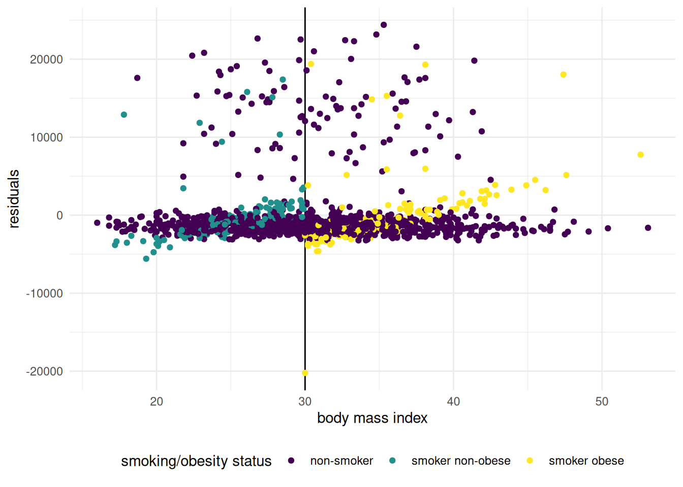
Figure 2.10: Residuals from the interaction model for \(\texttt{charges}\) with \(\texttt{age}\), \(\texttt{smoker}\) and \(\texttt{obesity}\). There is a notably outlier for a male smoker whose \(\texttt{bmi}\) is exactly 30 and other points above. There is indication of a linear trend for both smoker sub-groups as their body mass index increase, which was not apparent previously because of the effect of age.

2.7.1 Two-way ANOVA

“We’re the same as regression, but we’ve established a separate persona.” — Chelsea Parlett-Pelleriti

Two-way analysis of variance is a linear regression model with two categorical variables, and possibly an interaction term between the two. We consider a study on the effect of the type of delay and source of delay on the evaluation of service and on time lost waiting.

Hui, M. K., Thakor, M. V. et Gill, R. (1998). The Effects of Delay Type and Service Stage on Consumers’ Reaction to Waiting. Journal of Consumer Research 24, 469-479.

In a university, 120 participants tried a new course registration system. They were actually using a fake registration system where factors of interest could be manipulated, the advancement stage in the registration process and the type of delay. The two levels for stage of advancement were close to end and far from end. In stage far from end, a message indicating a delay appeared immediately at the beginning of the registration process. For the stage close to end, the delay message appeared after the participant has entered personal information and course choices.

There were three types of delays: procedural, correctional, and unknown. The delay message indicated that the server was currently busy (procedural delay), that there were problems with the terminal and that the system needed to reestablish the connection (correctional delay) or else simply stated “please wait” (unknown delay).

At the end of the registration process, the participants were asked to estimate the delay time (in minutes) incurred during the registration process. They were also asked to provide an evaluation of the service using two measurement scales. The simulated data corresponding to this study are found in the \(\texttt{delay}\) database, which contains the following variables

• \(\texttt{time}\): delay time (in minutes) according to the participant.
• \(\texttt{eval}\): evaluation of service (standardized score).
• \(\texttt{stage}\): stage of advancement, a factor with levels close to end and far from end
• \(\texttt{delay}\): type of delay, a factor with levels procedural, correctional and unknown.

In the experimental design, the 120 participants were randomly assigned to one of these six conditions, but nine of the 120 participants were removed because they were not able to specify the type of delay that occurred. The dataset is unbalanced, meaning that the number of observations in each cell is unequal. If there had been the same number of observations in each subgroup for factors \(A\), \(B\), the test for the effect of factor \(A\) given that \(B\) is already in the model would be the same as the marginal effect of \(A\) only.

We will evaluate the effect of the factors \(\texttt{delay}\) and \(\texttt{stage}\) on the estimated waiting time.

If there is an interaction between explanatory variables, but the latter is not included in the models, the tests are misleading: one assumption of the linear model being that all of the relevant covariates have been included and their effect properly accounted for. In this example, omitting the interaction leads to effects being averaged and cancelling each other. Fitting an ANOVA model with only additive (main effects, without interaction) for the evaluation of service suggests that the factors \(\texttt{stage}\) and \(\texttt{delay}\) are not significant: the \(p\)-values for the main effects, reported in Table 2.6, are \(0.409\) and \(0.137\). Therefore, there seemingly is no significant difference in delay time between the two stages and the three delay types.

Table 2.6: Analysis of variance table (Type 3 sum of square decomposition table) for the model for evaluation of service without interaction. While both factor appear not to be significant given the other, interaction plots show this is due to cancellation effects. The conclusions of the test are invalid because model assumptions are violated.

variable	sum of square	df	F stat.	p-value
(Intercept)	0	1	0.11	0.74
stage	0.3	1	0.69	0.41
delay	1.6	2	2.02	0.14
Residuals	41.9	105

However, looking at the data and the mean of each sub-class paints a different portrait, as evidenced by the interaction plot of Figure 2.11. The score for service increases for correctional delays when the error occurs close to the end, but the effect is opposite for other delay types. The fact that our \(p\)-values for the effects were not significative merely indicate that the effects cancelled out each other.

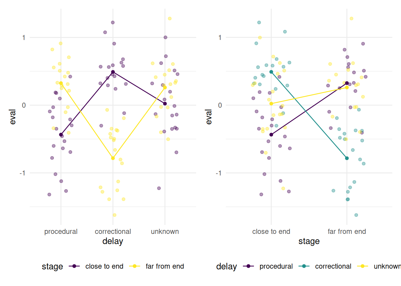
Figure 2.11: Interactions plots for the \(\texttt{delay}\) data, with jitterd observations: if there was no interaction, the curves should be parallel. These plots seem to indicate an interaction.

There is a significant interaction between the variables \(\texttt{delay}\) and \(\texttt{stage}\) on evaluation. Therefore, the effect of \(\texttt{delay}\) on the variable \(\texttt{eval}\) depends on the level of the variable \(\texttt{stage}\) ance vice-versa. Since there is an interaction term, tests for the main effects of \(\texttt{stage}\) or \(\texttt{delay}\) are not of interest.

Table 2.7: Analysis of variance table (Type 3 sum of square decomposition table). The only test of interest is that for the interaction, which is highly significant.

variable	sum of square	df	F stat.	p-value
(Intercept)	3.8	1	18.29	< 0.001
stage	5.3	1	25.67	< 0.001
delay	8.1	2	19.64	< 0.001
stage:delay	20.5	2	49.63	< 0.001
Residuals	21.3	103

If a difference is detected at this stage, one could then proceed to compute all pairwise differences within a given level of the other categorical variable. This is equivalent to running multiple \(t\)-tests, but the linear model assumes equal variance and would thus pool all observations to estimate the latter. For example, we could test if the difference between procedural and correctional delays when the error occurs far from the end of the procedure is significant. The mean differences of a factor for a given level of another factor are called simple effects. If the interaction is significant, there must be at least one pairwise difference which is also significant. However, repeated testing can inflate the Type I error, as illustrated in this comic strip: if we conduct 20 independent tests and the null is true in all cases (so there are no difference between any of the sub-groups), we would still expect to reject (by mistake) 1/20 on average for tests performed at level \(\alpha\). There exists method to adjust for multiple testing.

While the normality assumption is less crucial for the reliability of the tests, it requires sufficient sample size in each subgroup for these (say 20), so that the central limit theorem kicks in. The tests and models typically use the pooled variance estimators: in small samples, it makes better use of the data and has higher precision than estimators of the individual variance in each subgroups. If the variance were unequal, comparisons would require extended models covered later in the term and pairwise comparisons could be based on Welch test statistic.

2.8 Collinearity

The linearity assumption can be interpreted broadly to mean that all relevant covariates have been included and that their effect is correctly specified in the equation of the mean. Adding superfluous covariates to a model has limited impact: if the (partial) correlation between a column vector \(\mathbf{X}_k\) and the response variable \(\boldsymbol{Y}\) is zero, then \(\beta_k=0\) and the estimated coefficient \(\widehat{\beta}_k \approx 0\) because the least square estimators are unbiased. If we include many useless variables, say \(k\), the lack of parsimony can however make interpretation more difficult. The price to pay for including the \(k\) additional covariates is an increase in the variance of the estimators \(\widehat{\boldsymbol{\beta}}\).

It is nevertheless preferable to include more variables than to forget key predictors: if we omit an important predictor, their effect may be picked up by other regressors (termed confounders) in the model with are correlated with the omitted variable. The interpretation of the other effects can be severely affected by confounders. For example, the simple linear model (or two-sample \(t\)-test) for salary as a function of sex for the college data is invalid because sex is a confounder for rank. Since there are more men than women full professor, the mean salary difference between men and women is higher than it truly is. One way to account for this is to include control variables (such as rank), whose effect we need not be interested in, but that are necessary for the model to be adequate. We could also have used stratification, i.e., tested for wage discrimination within each academic rank. This is the reason why sociodemographic variables (sex, age, education level, etc.) are collected as part of studies.

A linear model is not a causal model: all it does is capture the linear correlation between an explanatory variable and the response. When there are more than one explanatory, the effect of \(\mathrm{X}_j\) given what has not already been explained by \(\mathbf{X}_{-j}\). Thus, if we fail to reject \(\mathscr{H}_0:\beta_j=0\) in favor of the alternative \(\mathscr{H}_1: \beta_j \neq 0\), we can only say that there is no significant linear association between \(\mathrm{X}_j\) and \(Y\) once the effect of other variables included in the model has been accounted for. There are thus two scenarios: either the response is uncorrelated with \(\mathrm{X}_j\) (uninteresting case, but easy to pick up by plotting both or computing linear correlation), or else there is a strong correlation between \(\mathrm{X}_j\) and both the response \(Y\) as well as (some) of the other explanatory variables \(\mathrm{X}_1, \ldots, \mathrm{X}_p\). This problem is termed (multi)collinearity.

One potential harm of collinearity is a decrease in the precision of parameter estimators. With collinear explanatories, many linear combinations of the covariates represent the response nearly as well. Due to the (near) lack of identifiability, the estimated coefficients become numerically unstable and this causes an increase of the standard errors of the parameters. The predicted or fitted values are unaffected. Generally, collinearity leads to high estimated standard errors and the regression coefficients can change drastically when new observations are included in the model, or when we include or remove explanatories. The individual \(\beta\) coefficients may not be statistically significant, but the global \(F\)-test will indicate that some covariates are relevant for explaining the response. This however would also be the case if there are predictors with strong signal, so neither is likely to be useful to detect issues.

The added-variable plot shows the relation between the response \(Y\) and an explanatory \(\mathrm{X}_j\) after accounting for other variables: the slope \(\widehat{\beta}_j\) of the simple linear regression is the same of the full model. A similar idea can be used to see how much of \(\mathrm{X}_j\) is already explained by the other variables. For a given explanatory variable \(\mathrm{X}_j\), we define its variance inflation factor as \(\mathsf{VIF}(j)=(1-R^2(j))^{-1}\), where \(R^2(j)\) is the coefficient of determination of the model obtained by regressing \(\mathrm{X}_j\) on all the other explanatory variables, i.e., \[\begin{align*} \mathrm{X}_j = \beta^{\star}_0 + \beta^{\star}_1 \mathrm{X}_1 + \cdots + \beta^{\star}_{j-1} \mathrm{X}_{j-1} + \beta^{\star}_{j+1} \mathrm{X}_{j+1} + \cdots + \beta^{\star}_p\mathrm{X}_p + \varepsilon^{\star} \end{align*}\] By definition, \(R^2(j)\) represents the proportion of the variance of \(\mathrm{X}_j\) that is explained by all the other predictor variables. Large variance inflation factors are indicative of problems (typically covariates with \(\mathsf{VIF}>10\) require scrutinity, and values in the hundreds or more indicate serious problems).

Added-variable plots can also serve as diagnostics, by means of comparison of the partial residuals with a scatterplot of the pair \((Y, \mathrm{X}_j)\); if the latter shows very strong linear relation, but the slope is nearly zero in the added-variable plot, this hints that collinearity is an issue.

What can one do about collinearity? If the goal of the study is to develop a predictive model and we’re not interested in the parameters themselves, then we don’t need to do anything. Collinearity is not a problem for the overall model: it’s only a problem for the individual effects of the variables. Their joint effect is still present in the model, regardless of how the individual effects are combined.

If we are interested in individual parameter estimates, for example, to see how (and to what extent) the predictor variables explain the behaviour of \(Y\), then things get more complicated. Collinearity only affects the variables that are strongly correlated with one another, so we only care if it affects one or more of the variables of interest. There sadly is no good solution to the problem. One could

• try to obtain more data, so as to reduce the effects of collinearity appearing in specific samples or that are due to small sample size.
• create a composite score by somehow combining the variables showing collinearity.
• remove one or more of the collinear variables. You need to be careful when doing this not to end up with a misspecified model.
• use penalized regression. If \(\mathbf{X}^\top\mathbf{X}\) is (nearly) not invertible, this may restore the uniqueness of the solution. Penalties introduce bias, but can reduce the variance of the estimators \(\boldsymbol{\beta}\). Popular choices include ridge regression (with an \(l_2\) penalty), lasso (\(l_1\) penalty), but these require adjustment in order to get valid inference.

Whatever the method, it’s important to understand that it can be very difficult (and sometimes impossible) to isolate the individual effect of a predictor variable strongly correlated with other predictors.

Example 2.3 (Collinearity in the $\texttt{college}$ data) We consider the college data analysis and include all the covariates in the database, including years, the number of years since PhD. One can suspect that, unless a professor started his or her career elsewhere before moving to the college, they will have nearly the same years of service. In fact, the correlation between the two variables, service and years is r cor(college$service, college$years). The variance inflation factor for the five covariates

For categorical variables, the variance inflation factor definition would normally yield for each level a different value; an alternative is the generalized variance inflation factor (Fox and Monette 1992). Here, we are interested in gender disparities, so the fact that both service and field are strongly correlated is not problematic, since the \(\mathsf{VIF}\) for \(\texttt{sex}\) is not high and the other variables are there to act as control and avoid confounders.

Table 2.8: (Generalized) variance inflation factor for the \(\texttt{college}\) data.

service	years	rank	sex	field
5.92	7.52	2.01	1.03	1.06

2.9 Graphical analysis of residuals

So far, we have fit models and tested significance of the parameters without checking the model assumptions. The correctness of statements about the \(p\)-values and confidence intervals depend on the (approximate) validity of the model assumptions, which all stem from the distributional assumption for the error, assumed to be independent and identically distributed with \(\varepsilon_i \stackrel{\cdot}{\sim} \mathsf{No}(0, \sigma^2)\). This compact mathematical description can be broken down into four assumptions.

• normality of the errors
• linearity: the mean of \(Y\) is \(\beta_0 + \beta_1\mathrm{X}_1 + \cdots + \beta_p \mathrm{X}_p\).
• homoscedasticity: the error variance is constant
• independence of the errors.

This section reviews the assumptions made in order to allow statistical inference using the linear model and different residuals that serve as building blocks for graphical diagnostics. We investigate the consequences of violation of these assumptions and outline potential mitigation strategies, many of which are undertaken in other chapters.

When we perform an hypothesis test, we merely fail to reject the null hypothesis, either because the latter is true or else due to lack of evidence. The same goes for checking the validity of model assumptions: scientific reasoning dictates that we cannot know for certain whether these hold true. Our strategy is therefore to use implications of the linear model assumptions to create graphical diagnostic tools, so as to ensure that there is no gross violation of these hypothesis. However, it is important to beware of over-interpreting diagnostic plots: the human eye is very good at finding spurious patterns.

Other good references for the material in this section is:

• Forecasting: Principles and Practice, section 5.3

2.9.1 Residuals

Residuals are predictions of the errors \(\varepsilon\) and represent the difference between the observed value \(Y_i\) and the estimated value on the line. The ordinary residuals are \[\begin{align*} e_i=Y_i-\widehat{Y}_i, \qquad i =1, \ldots, n. \end{align*}\] The sum of the ordinary residuals is always zero by construction if the model includes an intercept, meaning \(\overline{e} = 0\).

Not all observations contribute equally to the adjustment of the fitted hyperplane. The geometry of least squares shows that the residuals are orthogonal to the fitted values, and \(\boldsymbol{e} = (\mathbf{I}_n-\mathbf{H}_{\mathbf{X}})\boldsymbol{Y}\), where \(\mathbf{H}_{\mathbf{X}}=\mathbf{X}(\mathbf{X}^\top\mathbf{X})^{-1}\mathbf{X}^\top\) is an \(n \times n\) projection matrix that spans the \(p\)-dimensional linear combination of the columns of \(\mathbf{X}\), \(\mathcal{S}(\mathbf{X})\). If \(\mathsf{Va}(\boldsymbol{Y}) = \sigma^2\mathbf{I}_n\), it follows that \(\mathsf{Va}(\boldsymbol{e})=\sigma^2(\mathbf{I}_n-\mathbf{H}_{\mathbf{X}})\) because \((\mathbf{I}_n-\mathbf{H}_{\mathbf{X}})\) is a projection matrix, therefore idempotent and symmetric. Because the matrix has rank \(n-p\), the ordinary residuals cannot be independent from one another.

If the errors are independent and homoscedastic, the ordinary residual \(e_i\) has variance \(\sigma^2(1-h_{i})\), where the leverage term \(h_i =(\mathbf{H}_{\mathbf{X}})_{ii} = \mathbf{x}_i (\mathbf{X}^\top\mathbf{X})^{-1}\mathbf{x}_i\) is the \(i\)th diagonal entry of the projection matrix \((\mathbf{H}_{\mathbf{X}})\) and \(\mathbf{x}_i\) is the \(i\)th row of the model matrix corresponding to observation \(i\).

We thus conclude that ordinary residuals do not all have the same standard deviation and they are not independent. This is problematic, as we cannot make meaningful comparisons: points with low leverage are bound to deviate more from the fitted model than others. To palliate to this, we can standardize the residuals so each has the same variance under the null of independent homoscedastic errors — the leverage terms \(h_i\) are readily calculated from the model matrix \(\mathbf{X}\). The only remaining question is how to estimate the variance. If we use the \(i\)th observation to estimate both the residual and the variance, we introduce additional dependence. A better way is remove the \(i\)th observation and refit the model with the \(n-1\) remaining observations to get of \(s^2_{(-i)}\) (there are tricks and closed-form expressions for these, so one doesn’t need to fit \(n\) different linear models). The jacknife studentized residual \(r_i = e_i/\{s_{(-i)}(1-h_i)\}\), also termed externally studentized residuals, are not independent, but they are identically distributed and follow a Student distribution with \(n-p-2\) degrees of freedom. These can be obtained in R with the command rstudent, also in SAS.

When to use which residuals? By construction, the vector of ordinary residuals \(\boldsymbol{e}\) is orthogonal to the fitted values \(\widehat{\boldsymbol{y}}\) and also to each column of the model matrix \(\mathbf{X}\): this means a simple linear regression of \(\boldsymbol{e}\) with any of these as covariate gives zero intercept and zero slope. However, residual patterns due to forgotten interactions, nonlinear terms, etc. could be picked up from pair plots of ordinary residuals against the explanatories.

While the jackknife studentized residuals \(r_i\) are not orthogonal, they are not very different. Use jackknife residuals \(\boldsymbol{r}\) to check for equality of variance and distributional assumptions (e.g., using quantile-quantile plots).

One thus typically uses ordinary residuals \(\boldsymbol{e}\) for plots of fitted values/explanatories against residuals and otherwise jackknife studentized residuals for any other graphical diagnostic plot.

2.9.2 Leverage and outliers

The leverage \(h_i\) of observation \(i\) measures its impact on the least square fit, since we can write \(h_i = \partial \widehat{y}_i/\partial y_i\). Leverage values tell us how much each point impacts the fit: they are strictly positive, are bounded below by \(1/n\) and above by \(1\). The sum of the leverage values is \(\sum_{i=1}^n h_i=p+1\): in a good design, each point has approximately the same contribution, with average weight \((p+1)/n\).

Points with high leverage are those that have unusual combinations of explanatories. An influential observation (\(h_i\approx 1\)) pulls the fitted hyperplane towards itself so that \(\hat{y}_i \approx y_i\). As a rule of thumb, points with \(h_i> 2(p+1)/n\) should be scrutinized.

It is important to distinguish betwen influential observations (which have unusual \(\mathbf{x}\) value, i.e., far from the overall mean) and outliers (unusual value of the response \(y\)). If an observation is both an outlier and has a high leverage, it is problematic.

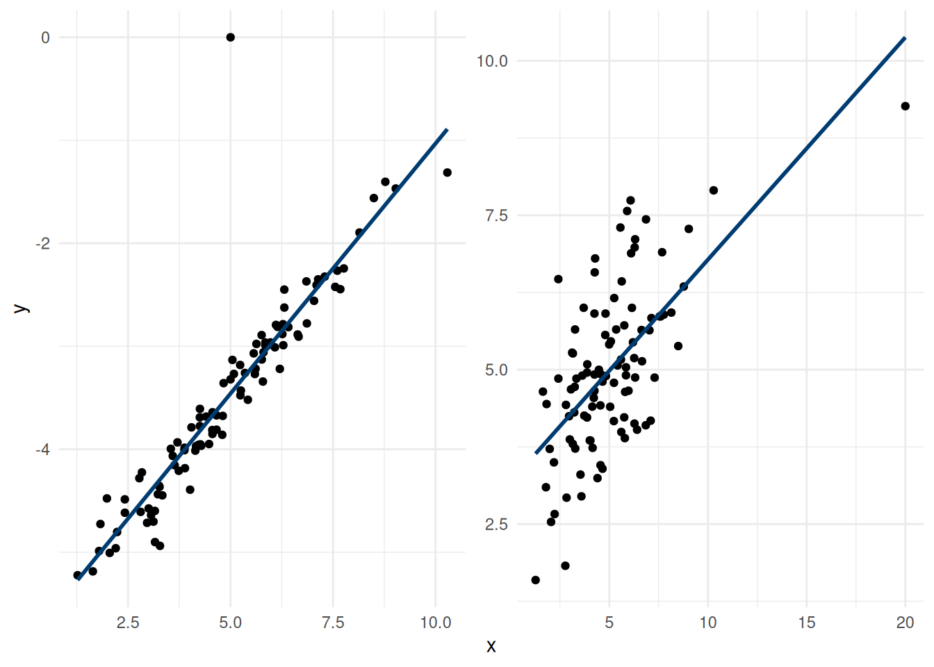
Figure 2.12: Outlier and influential observation. The left panel shows an outlier, whereas the right panel shows an influential variable (rightmost \(x\) value).

If influential observations can be detected by inspecting the leverage of each observation, outliers are more difficult to diagnose.

An outlier stands out from the rest of the observations, either because it has an usual response value, or because it falls far from the regression surface. Loosely speaking, an outlier is an unusual values of \(Y\) for a given combination of \(\mathbf{X}\) that ``stand out’’ from the rest. Outliers can be detected during the exploratory data analysis or picked-up in residual plots (large values of \(|e_i|\) in plots of fitted versus residuals) or added-variable plots. One could potentially test whether an jackknife studentized residual is an outlier (adjusting for the fact we would consider only largest values). One can also consider Cook’s distance, \(C_j\), a statistic giving the scaled distance between the fitted values \(\hat{\boldsymbol{y}}\) and the fitted values for the model with all but the \(j\)th observation, \(\hat{\boldsymbol{y}}^{(-j)}\), \[\begin{align*} C_j = \frac{1}{(p+1)S^2} \sum_{i=1}^n \left\{\hat{y}_i - \hat{y}_{i}^{(-j)}\right\}^2 \end{align*}\] Large values of \(C_j\) indicate that its residual \(e_j\) is large relative to other observations or else its leverage \(h_j\) is high. A rule of thumb is to consider points for which \(C_j > 4/(n-p-1)\). In practice, if two observations are outlying and lie in the same region, their Cook distance will be halved.

Outliers and influential observations should not be disregarded because they don’t comply with the model, but require further investigation. They may motivate further modelling for features not accounted for. It is also useful to check for registration errors in the data (which can be safely discarded).

Except in obvious scenarios, unusual observations should not be discarded. In very large samples, the impact of a single outlier is hopefully limited. Transformations of the response may help reduce outlyingness. Otherwise, alternative objective functions (as those employed in robust regression) can be used; these downweight extreme observations, at the cost of efficiency.

2.9.3 Diagnostic plots

We review the assumptions in turn and discuss what happens when the assumptions fail to hold.

2.9.3.1 Independence assumption

Usually, the independence of the observations follows directly from the type of sampling used — this assumption is implicitly true if the observations were taken from a random sample from the population. This is generally not the case for longitudinal data, which contains repeated measures from the same individuals across time. Likewise, time series are bound not to have independent observations. If we want to include all the time points in the analysis, we must take into account the possible dependence (correlation) between observations. If we ignore correlation, the estimated standard errors are too small relative to the truth, so the effective sample size is smaller than number of observations.

The first source of dependence is clustered data, meaning measurements taken from subjects that are not independent from one another (family, groups, etc.) More generally, correlation between observations arises from time dependence, roughly categorized into

• longitudinal data: repeated measurements are taken from the same subjects (few time points)
• time series: observations observed at multiple time periods (many time points). Time series require dedicated models not covered in this course.

Because of autocorrelation, positive errors tend to be followed by positive errors, etc. We can plot the residuals as a function of time, and a scatterplot of lagged residuals \(e_i\) versus \(e_{i-1}\) (\(i=2, \ldots, n\)).

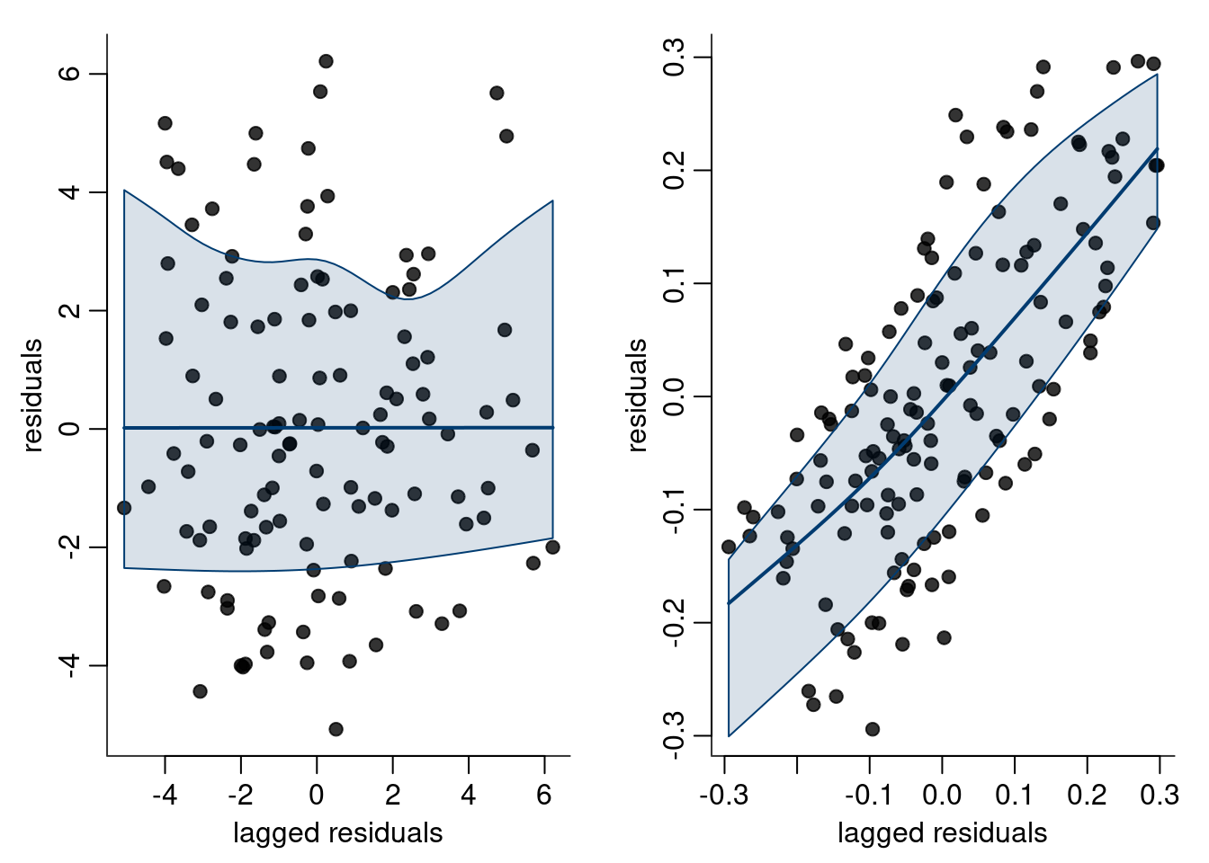
Figure 2.13: Lagged residual plots: there is no evidence against independence in the left panel, whereas the right panel shows positively correlated residuals.

However, lagged residuals plots only show dependence at lag one between observations. For time series, we can look instead at a correlogram, i.e., a bar plot of the correlation between two observations \(h\) units apart as a function of the lag \(h\) (Brockwell and Davis 2016, Definition 1.4.4).

For \(y_1, \ldots, y_n\) and constant time lags \(h=0, 1, \ldots\) units, the autocorrelation at lag \(h\) is \[\begin{align*} r(h) = \frac{\gamma(h)}{\gamma(0)}, \qquad \gamma(h) = \frac{1}{n}\sum_{i=1}^{n-|h|} (y_i-\overline{y})(y_{i+h}) - \overline{y}) \end{align*}\]

If the series is correlated, the sample autocorrelation will likely fall outside of the pointwise confidence intervals, as shown in Figure 2.14. Presence of autocorrelation requires modelling the correlation between observations explicitly using dedicated tools from the time series literature that are covered in MATH 60638. We will however examine \(\mathsf{AR}(1)\) models as part of the chapter on longitudinal data.

When observations are positively correlated, the estimated standard errors reported by the software are too small. This means we are overconfident and will reject the null hypothesis more often then we should if the null is true (inflated Type I error, or false positive).

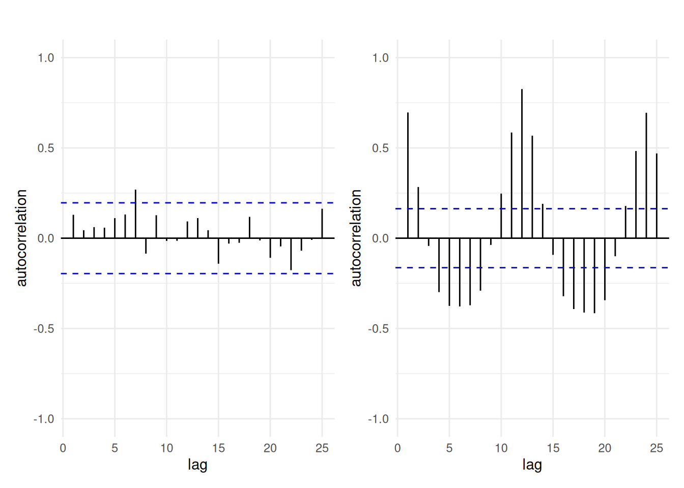
Figure 2.14: Correlogram of independent observations (left) and the ordinary residuals of the log-linear model fitted to the air passengers data (right). While the mean model of the latter is seemingly correctly specified, there is residual dependence between monthly observations and yearly (at lag 12). The blue lines give approximate pointwise 95% confidence intervals for white noise (uncorrelated observations).

2.9.3.2 Linearity assumption

The second assumption of the linear model is that of linearity, which means that the mean model is correctly specified, all relevant covariates have been included and their effect is correctly specified. To check that the response surface of the linear model is adequate, we plot \(e_i\) against \(\widehat{y}_i\) or \(\mathrm{X}_{ij}\) (for \(j=1, \ldots, p\)). Since the linear correlation between \(\boldsymbol{e}\) and \(\widehat{\boldsymbol{y}}\) (or \(\boldsymbol{e}\) and \(\mathbf{X}_j\)) is zero by construction, patterns (e.g., quadratic trend, cycles, changepoints) are indicative of misspecification of the mean model. One can add a smoother to detect patterns. Figure 2.15 shows three diagnostics plots, the second of which shows no pattern in the residuals, but skewed fitted values.

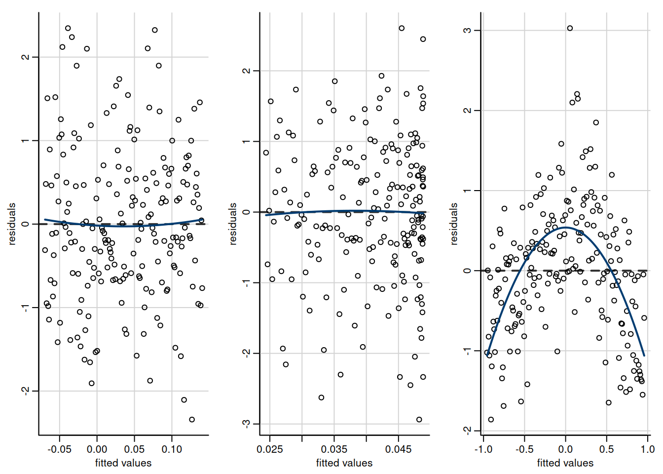
Figure 2.15: Scatterplots of residuals against fitted values. The first two plots show no departure from linearity (mean zero). The third plot shows a clear quadratic pattern, suggesting the mean model is misspecified. Note that the distribution of the fitted value need not be uniform, as in the second panel which shows more high fitted values.

If there is residual structure in plots of ordinary residuals against either (a) the fitted values or (b) the explanatory variables, a more complex model can be adjusted including interactions, nonlinear functions, If the effect of an explanatory variable is clearly nonlinear and complicated, smooth terms could be added (we won’t cover generalized additive models in this course).

Plotting residuals against left-out explanatory variables can also serve to check that all of the explanatory power of the omitted covariate is already explained by the columns of \(\mathbf{X}\).

If an important variable has been omitted and is not available in the dataset, then the effect of that variable is captured by both the errors (the portion orthogonal to the model matrix \(\mathbf{X}\), i.e., unexplained by the covariates included in the model) and the remaining part is captured by other explanatories of the model that are correlated with the omitted variable. These variables can act as confounders. There is little that can be done in either case unless the data for the omitted variable are available, but subject-specific knowledge may help make sense of the results.

2.9.3.3 Homoscedasticity assumption

If the variance of the errors is the same for all observations, that of the observations \(Y\) is also constant. The most common scenarios for heteroscedasticity are increases in variance with the response, or else variance that depends on explanatory variables \(\mathbf{X}\), most notably categorical variables. For the former, a log-transform (or Box–Cox transformation) can help stabilize the variance, but we need the response to be positive. For the latter, we can explicitly model that variance and we will see how to include different variance per group later on. A popular strategy in the econometrics literature, is to use robust (inflated) estimators of the standard errors such as White’s sandwich estimator of the variance.

If the residuals (or observations) are heteroscedastic (non constant variance), the estimated effects of the variables (the \(\beta\) parameters) are still valid in the sense that the ordinary least squares estimator \(\widehat{\boldsymbol{\beta}}\) is unbiased. However, the estimated standard errors of the \(\widehat{\beta}\) are no longer reliable and, consequently, the confidence intervals and the hypothesis tests for the model parameters will be incorrect. Indeed, if the variance of the errors differs from one observation to the next, we will estimate an average of the different variance terms. The standard errors of each term are incorrect (too small or too large) and the conclusions of the tests (\(p\)-values) will be off because the formulas of both \(t\)-test and \(F\)-test statistics include estimates of \(\hat{\sigma}^2\).

Looking at the plot of jackknife studentized residuals against regressors (or fitted values) is instructive — for example, we often see a funnel pattern when there is an increase in variance in the plot of the jackknife studentized residuals against fitted value, or else in boxplots with a categorical variable as in Figure 2.17. However, if we want to fit a local smoother to observe trends, it is better to plot the absolute value of the jackknife studentized residuals against regressors or observation number.

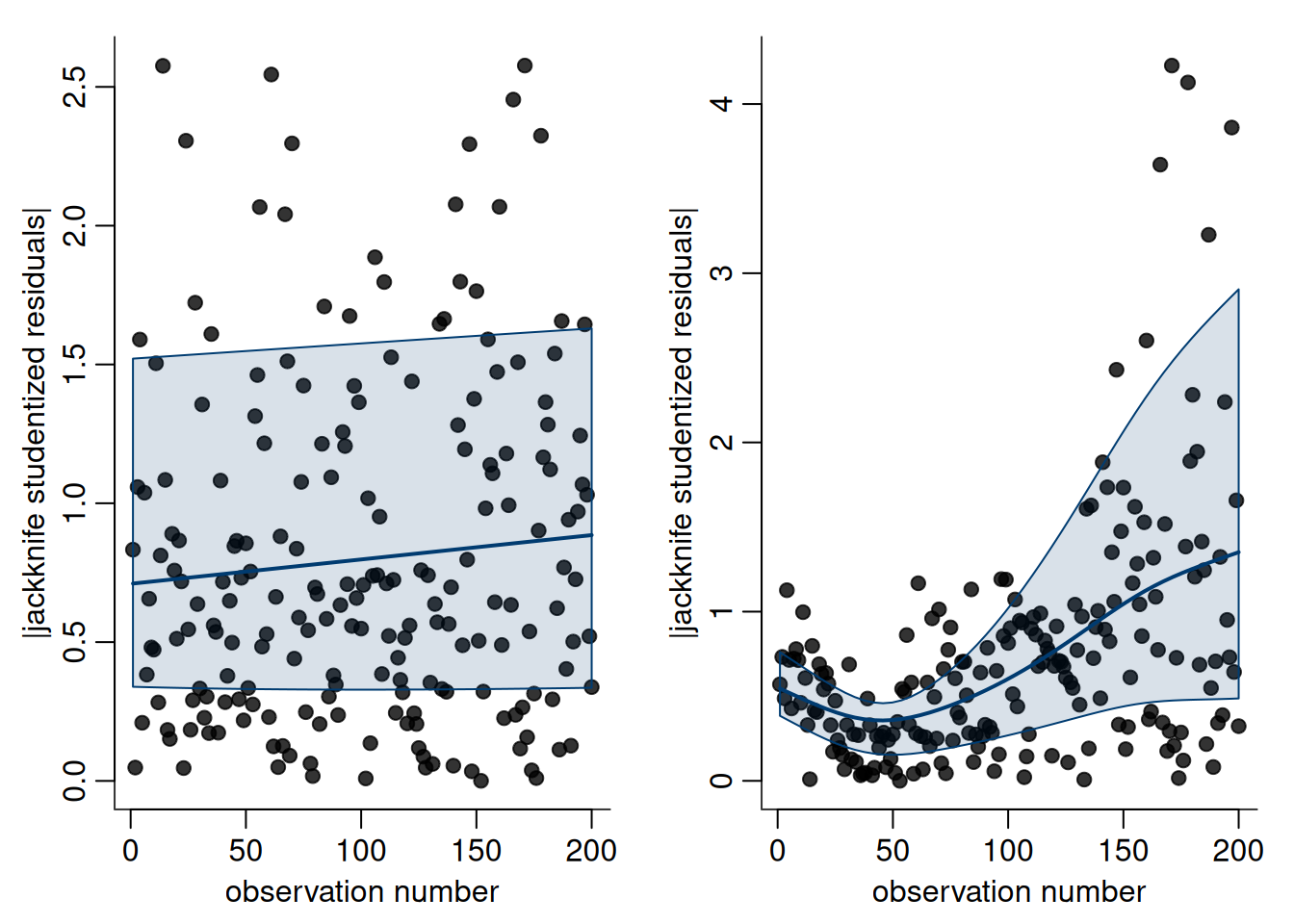
Figure 2.16: Plot of the absolute value of jackknife studentized residuals against observation number. The left panel is typical of homoscedastic data, whereas the right panel indicates an increase in the variance.

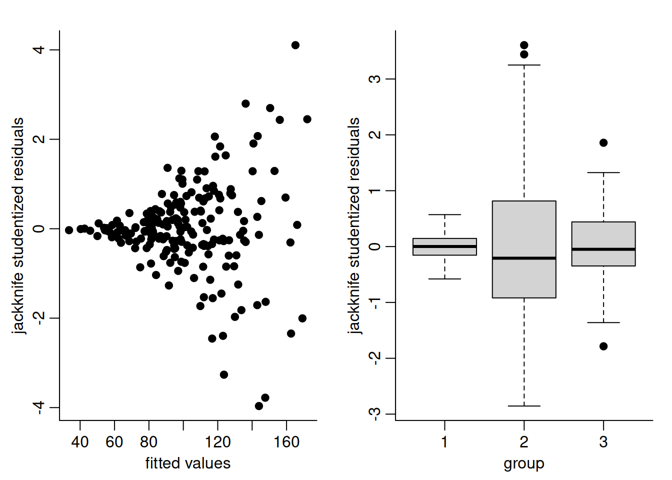
Figure 2.17: Plot of jackknife studentized residuals against fitted value (left) and categorical explanatory (right). Both clearly display heteroscedasticity.

2.9.3.4 Normality assumption

The normality assumption is mostly for convenience: if the errors are assumed normally distributed, then the least square and the maximum likelihood estimators of \(\boldsymbol{\beta}\) coincide. The maximum likelihood estimators of \(\boldsymbol{\beta}\) are asymptotically normal under mild conditions on the model matrix and \(t\)-tests are robust to departure of the normality assumption. This means that inference is valid in large samples, regardless of the distribution of the errors/residuals (even if the null distribution are not exact). It is important to keep in mind that, for categorical explanatory variables, the sample size in each group must be sufficiently large for the central limit theorem to kick in.

Sometimes, transformations can improve normality: if the data is right-skewed and the response is strictly positive, a log-linear model may be more adequate. This can be assessed by looking at the quantile-quantile plot of the externally studentized residuals. If the response \(Y\) is not continuous (including binary, proportion or count data), linear models give misleading answers and generalized linear models are more suitable.

The inference will be valid for large samples even if the errors are not normally distributed by virtue of the central limit theorem. If the errors \(\varepsilon_i \sim \mathsf{No}(0, \sigma^2)\), then the jacknnife studentized residuals should follow a Student distribution, with \(r_i \sim \mathsf{St}(n-p-2)\), (identically distributed, but not independent). A Student quantile-quantile plot can thus be used to check the assumption (and for \(n\) large, the normal plotting positions could be used as approximation if \(n-p> 50\)). One can also plot a histogram of the residuals. Keep in mind that if the mean model is not correctly specified, some residuals may incorporate effect of leftover covariates.

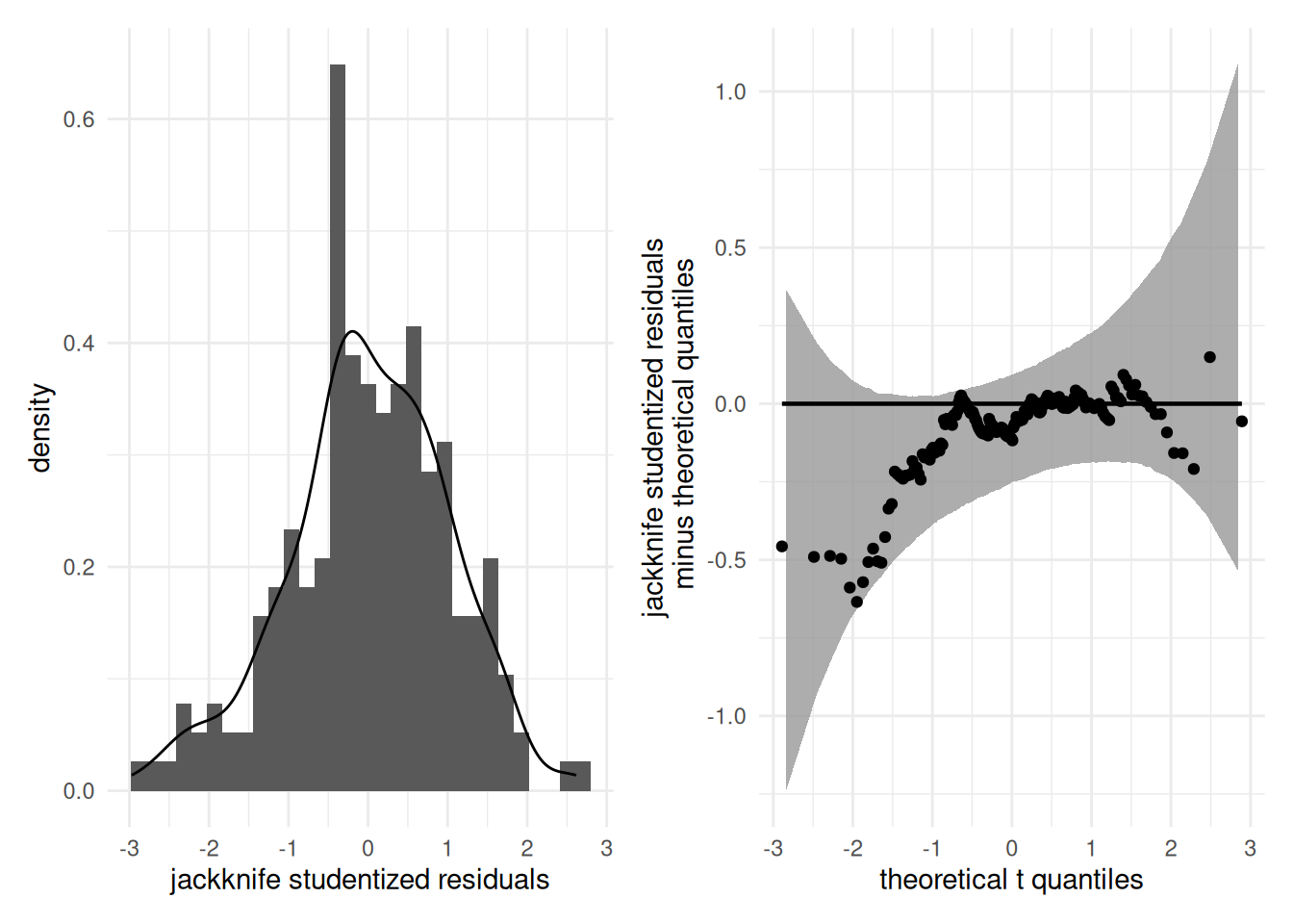
Figure 2.18: Histogram (left) and Student quantile-quantile plot (right) of the jackknife studentized residuals. The left panel includes a kernel density estimate (black), with the density of Student distribution (blue) superimposed. The right panel includes pointwise 95% confidence bands calculated using a bootstrap.

Quantile-quantile plots are discussed in Section A.2.5, but their interpretation requires training. For example, Figure 2.19 shows many common scenarios that can be diagnosed using quantile-quantile plots: discrete data is responsible for staircase patterns, positively skewed data has too high low quantiles and too low high quantiles relative to the plotting positions, heavy tailed data have high observations in either tails and bimodal data leads to jumps in the plot.

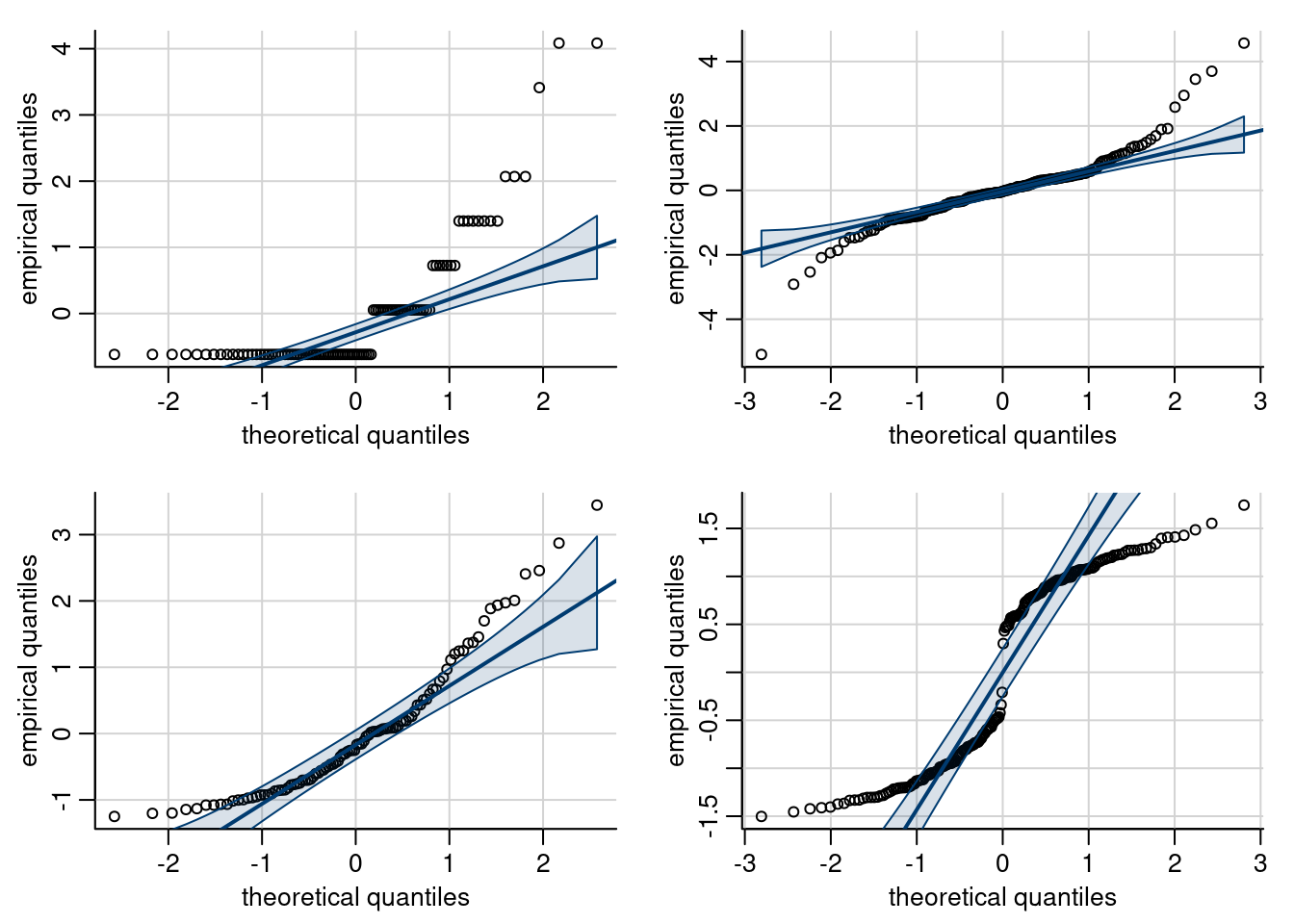
Figure 2.19: Quantile-quantile plots of non-normal data, showing typical look of behaviour of discrete (top left), heavy tailed (top right), skewed (bottom left) and bimodal data (bottom right).

Example 2.4 (Diagnostic plots for the $\texttt{college}$ data.) We can look at the college data to see if the linear model assumptions hold.

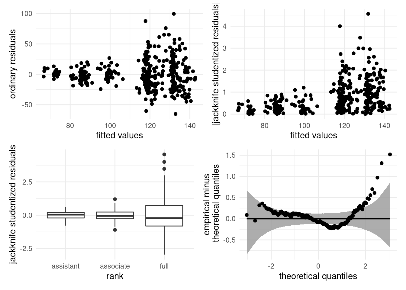
Figure 2.20: Diagnostic plots for the college data example: ordinary residuals against fitted values (top left), absolute value of the jacknnife studentized residuals against fitted values (top right), box and whiskers plot of jacknnife studentized residuals (bottom left) and detrended Student quantile-quantile plot (bottom right). There is clear group heteroscedasticity.

Based on the plots of Figure 2.20, we find that there is residual heteroscedasticity, due to rank. Since the number of years in the first rank is limited and all assistant professors were hired in the last six years, there is less disparity in their income. It is important not to mistake the pattern on the \(x\)-axis for the fitted value (due to the large effect of rank and field, both categorical variable) with patterns in the residuals (none apparent). Fixing the heteroscedasticity would correct the residuals and improve the appearance of the quantile-quantile plot.

2.10 Transformation of the response

This ultimate section deals with strategies for fixing the linear model if we detected non-normality. If the response is strictly positive, an option is to use the Box–Cox transformation presented in Section 3.3 and fit a linear model to a transformation of \(Y\), \[\begin{align*} y_i(\lambda)= \begin{cases} (y^{\lambda}-1)/\lambda, & \lambda \neq 0\\ \ln(y), & \lambda=0. \end{cases} \end{align*}\] We then fit a linear model over a grid of \(\lambda\), using the profile likelihood to select the optimal value for the transformation. Note that the latter will depend on the covariates present in the model; the example with the \(\texttt{college}\) data already shows that the diagnostics of normality is impacted by departures from the other hypothesis. The cases \(\lambda=1\) (identity) and \(\lambda=0\) (log-linear model) are perhaps the most important because they yield interpretable coefficients.

If the data is right-skewed and the response is strictly positive, a log-linear model may be more adequate and the parameters can be interpreted. Theory sometimes dictates a multiplicative model: for example, the Cobb–Douglas production function in economics is \(P=\alpha L^{\beta_1}C^{\beta_2}\), where \(P\) stands for production, \(L\) for labor and \(C\) for capital; all inputs are positive, so taking a log-transform yields a model that is linear in \(\beta\), with \(\beta_0=\ln(\alpha)\).

We can rewrite the model in the original response scale as \[\begin{align*} Y = \exp\left(\beta_0+\sum_{j=1}^p\beta_j\mathrm{X}_j + \varepsilon \right) = \exp\left(\beta_0+ \sum_{j=1}^p\beta_j\mathrm{X}_j\right)\cdot \exp(\varepsilon), \end{align*}\] and thus \[\begin{align*} \mathsf{E}(Y \mid \mathbf{X}) = \exp(\beta_0 +\beta_1 \mathrm{X}_1 +\cdots + \beta_p\mathrm{X}_p ) \times \mathsf{E}\{\exp(\varepsilon) \mid \mathbf{X}\}. \end{align*}\] If \(\varepsilon \mid \mathbf{X} \sim \mathsf{No}(\mu,\sigma^2)\), then \(\mathsf{E}\{\exp(\varepsilon) \mid \mathbf{X}\}= \exp(\mu+\sigma^2/2)\) and \(\exp(\varepsilon)\) follows a log-normal distribution.

In order to interpret the parameters, we can compare the ratio of \(\mathsf{E}(Y \mid \mathrm{X}_1=x+1)\) to \(\mathsf{E}(Y \mid \mathrm{X}_1=x)\), \[\begin{align*} \frac{\mathsf{E}(Y \mid \mathrm{X}_1=x+1, \mathrm{X}_2, \ldots, \mathrm{X}_p)}{\mathsf{E}(Y \mid \mathrm{X}_1=x, \mathrm{X}_2, \ldots, \mathrm{X}_p)} = \frac{\exp\{\beta_1(x+1)\}}{\exp(\beta_1 x)} = \exp(\beta_1). \end{align*}\] Thus, \(\exp(\beta_1)\) represents the ratio of the mean of \(Y\) when \(\mathrm{X}_1=x+1\) in comparison to that when \(\mathrm{X}_1=x\), ceteris paribus (and provided this statement is meaningful). We can interpret \(\exp(\beta_1)\) as the multiplicative effect of \(\mathrm{X}_1\) on the mean of \(Y\): increasing \(\mathrm{X}_1\) by one unit causes \(Y\) to increase by a factor of \(\exp(\beta_1)\), on average.

Sometimes, we may wish to consider a log transformation of both the response and some of the continuous positive explanatories, when this make sense.

Consider the case where both \(Y\) and \(\mathrm{X}_1\) is log-transformed, so the equation for the mean on the original data scale reads \[\begin{align*} Y= \mathrm{X}_1^{\beta_1}\exp(\beta_0 + \beta_2\mathrm{X}_2 + \cdots + \beta_p\mathrm{X}_p + \varepsilon) \end{align*}\] Taking the derivative of the left hand side with respect to \(\mathrm{X}_1>0\), we get \[\begin{align*} \frac{\partial Y}{\partial \mathrm{X}_1}&= \beta_1 \mathrm{X}_1^{\beta_1-1}\exp(\beta_0 + \beta_2\mathrm{X}_2 + \cdots + \beta_p\mathrm{X}_p + \varepsilon) \\&= \frac{\beta_1 Y}{\mathrm{X}_1} \end{align*}\] and thus we can rearrange the expression so that \[\begin{align*} \frac{\partial \mathrm{X}_1}{\mathrm{X}_1}\beta_1 = \frac{\partial Y}{Y}; \end{align*}\] this is a partial elasticity, so \(\beta_1\) is interpreted as a \(\beta_1\) percentage change in \(Y\) for each percentage increase of \(\mathrm{X}_1\), ceteris paribus.

Example 2.5 The paper of Box and Cox consider survival time for 48 animals based on a randomized trial; these data are analyzed in Example 8.25 of Davison (2008). Three poisons were administered with four treatments; each factor combination contained four animals, chosen at random. There is strong evidence that both the choice of poison and treatment affect survival time.

We could consider a two-way analysis of variance model for these data without interaction, given the few observations for each combination. The model would be of the form \[\begin{align*} Y &= \beta_0 + \beta_1 \texttt{poison}_2 + \beta_2\texttt{poison}_3 +\beta_3\texttt{treatment}_2 \\ &\qquad+ \beta_4\texttt{treatment}_3 +\beta_5\texttt{treatment}_4 + \varepsilon \end{align*}\]

The plot of fitted values against residuals shows that the model is not additive; there is also indications that the variance increases with the mean response. The model is inadequate: lowest survival times are underpredicted, meaning the residuals are positive and likewise the middle responses is positive. A formal test of non-additivity based on constructed variables further point towards non-additivity (Davison 2008, Example 8.24). Overall, the model fit is poor and any conclusion drawn from it dubious.

One could consider using a Box–Cox to find a suitable transformation of the residuals so as to improve normality. The profile log likelihood at the bottom left of Figure 2.21 suggests that \(\lambda\approx -1\) would be a good choice. This has the benefit of being interpretable, as the reciprocal response \(Y^{-1}\) corresponds to the speed of action of the poison depending on both poison type and treatment. The diagnostics plots also indicate that the model for the reciprocal has no residual structure and the variance appears constant.

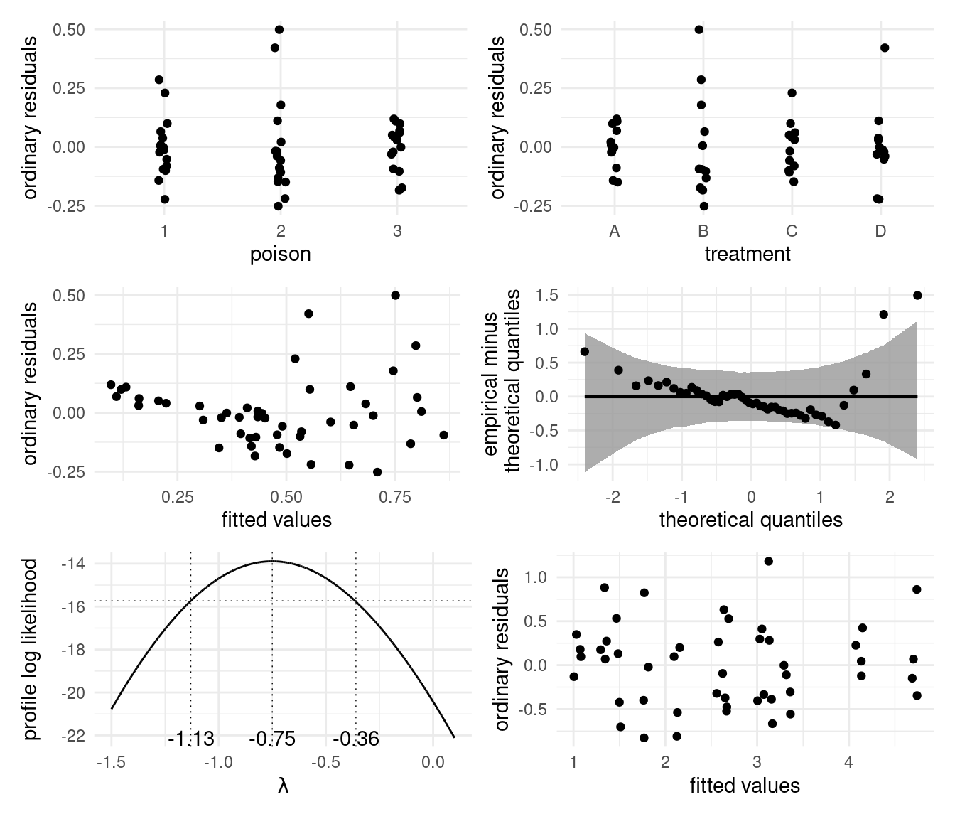
Figure 2.21: Diagnostic plots for the poison data. The top panel shows the ordinary residuals for the linear model for survival time as a function of poison and treatment, with jittered observations. The middle left plot shows the fitted values against residuals, which display evidence of trend and increase in variance with the survival time. The quantile-quantile plot in the middle right plot shows some evidence of departure from the normality, but the non-linearity and heteroscedasticity obscure this. The bottom panel shows the profile log likelihood for the Box–Cox transform, suggesting a value of \(-1\) would be within the 95% confidence interval. After fitting the same additive model with main effect only to the reciprocal survival time, there is no more evidence of residual structure and unequal variance.