6 Linear mixed models

A linear mixed model is a two-level hierarchical model of the form

\[\begin{align} \mathcal{B}_i &\sim \mathsf{No}_q(\boldsymbol{0}_q, \boldsymbol{\Omega}) \nonumber\\ \boldsymbol{Y}_i \mid \mathcal{B}_i=\boldsymbol{b}_i &\sim \mathsf{No}_{n_i}(\mathbf{X}_i\boldsymbol{\beta} + \mathbf{Z}_i\boldsymbol{b}_i, \mathbf{R}_i) \tag{6.1} \end{align}\] where \(i\) is the identifier of the group (clustered data) or individual (longitudinal data).

The \(n_i \times q\) model matrix \(\mathbf{Z}_i\) contains a subset of the columns of \(\mathbf{X}_i\). We term \(\mathbf{X}_i\boldsymbol{\beta}\) fixed effects and \(\mathbf{Z}_i\boldsymbol{b}\) random effects. The specification of (6.1) is particularly convenient for simulation: first sample a random effect vector \(\boldsymbol{b}_i\) common to the group, then simulate new responses whose mean is shifted by \(\mathbf{Z}_i\boldsymbol{b}_i\) relative to the linear regression. The matrix \(\mathbf{R}_i\) is typically the identity matrix \(\sigma^2\mathbf{I}_{n_i}\), but we could include slightly more general settings, including autoregressive errors.

Because the multivariate normal distribution, one can show that the joint distribution of \((\boldsymbol{Y}, \mathcal{B})\) is jointly normal, that the marginal response \(\boldsymbol{Y}_i\) is also normal. If we integrate out the random effect, \[\begin{align} \boldsymbol{Y}_i \sim \mathsf{No}_{n_i}( \mathbf{X}_i \boldsymbol{\beta}, \mathbf{Z}_i\boldsymbol{\Omega}\mathbf{Z}_i^\top + \mathbf{R}_i) \tag{6.2} \end{align}\]

In practice, we do not observe the random effect terms \(\boldsymbol{b}_i\), so the inclusion of random effects translates into a more complex covariance structure which is additive: one component, \(\mathbf{R}_i\), represents the covariance matrix of the random errors, while \(\mathbf{Z}_i\boldsymbol{\Omega}\mathbf{Z}_i^\top\) is the additional variability induced by random effects. We denote by \(\boldsymbol{\psi}\) the covariance parameters of \(\boldsymbol{\Sigma}_i= \mathbf{Z}_i\boldsymbol{\Omega}\mathbf{Z}_i^\top + \mathbf{R}_i\) and the fixed effect parameters \(\boldsymbol{\beta}\).

Parameter estimates are obtained from the likelihood of (??) and estimated using restricted estimation maximum likelihood (REML) or via maximum likelihood. In both cases, the optimization problems reduce to finding estimates of \(\boldsymbol{\psi}\) given that we an explicit solution for the restricted maximum likelihood parameters \[\begin{align*} \widehat{\boldsymbol{\beta}}_{\boldsymbol{\psi}} = (\mathbf{X}^\top\boldsymbol{\Sigma}^{-1}\mathbf{X})^{-1}\mathbf{X}^\top\boldsymbol{\Sigma}^{-1}\boldsymbol{Y} \end{align*}\] which is the generalized least square solutions.

6.1 Partial pooling

Random effects naturally induce correlation between observations and the conditional mean of \(\boldsymbol{Y}_i \mid \mathcal{B}_i\) includes a group-effect. The alternative is to include another fixed effect via an binary indicator of group, \(g_i\) and an interaction between time and group indicators, viz. \(g_i\cdot \texttt{time}\). There are many disadvantages to using this latter specification, since new observation or slope for incomplete records cannot be reliably estimated, in addition to having an overparametrized model with in addition no coefficients for explanatory variables that do not change within group.

Tristan Mahr masterfully illustrated in a blog post the shrinkage of random effects. The following section is adapted from his code (with the code hidden to streamline the argument).

Example 6.1 (Chicken growth curve) We consider for illustration the growth curves of chicken who are administered four different diets. The purpose of the study was to determine which diet was most effective for weight gain.

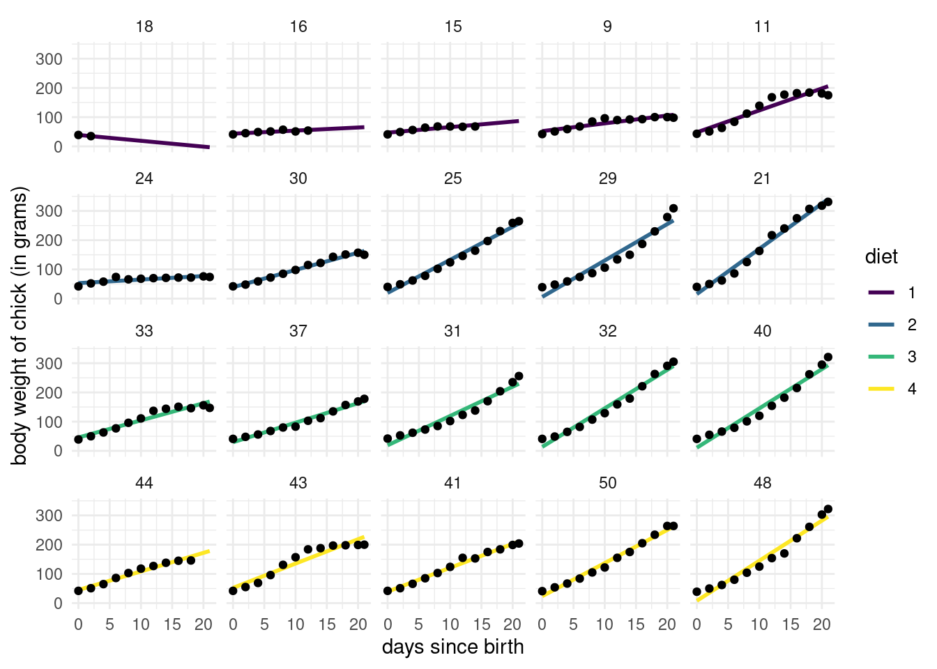
Figure 6.1: Chicken weight growth curve, ordered by weight. Each row corresponds to a different diet.

The spaghetti plot of Figure 6.1 shows selected individuals, ordered by their initial weight. We can see that some chicks are lost to follow-up, possibly dead, for the first diet type. While this is potentially a form of informative censoring, we will omit it from further analyses due to lack of additional information. Overall, the slopes seem steeper on average for diets 3–4. We omit diet from subsequent analyses, but including an interaction between age and diet, in addition to main effects, seems an adequate way to capture these differences. There are also variability within diet, as not all chicks have the same daily weight gain.

We can compare the group effect to a linear model with no pooling obtained by including a common slope for \(\texttt{time}\) in the model matrix \(\mathbf{X}\) and no group-specific intercept. This scenario corresponds to no pooling or “one size fits all”. This solution would differ slightly from the mixed model because it would simply pool all observations at a given time.

The main remaining question is related to discrepancies between conditional predictions from the mixed model with random intercepts and slopes and the model that includes fixed effects with different intercepts and slopes for each chick. It turns out that the specification of the normal random effects induces shrinkage towards zero of the random effect, and thus the conditional predictions (predictions of the random effects added to the fixed effects) are closer than their fixed effects counterparts, which is itself close to the global average intercept/slope. Most of the time, this effect is barely distinguishable in plots, as shown in Figure 6.2. The only exception seems to be in cases where the number of observations per group is small, in which case the conditional and marginal predictions are close.

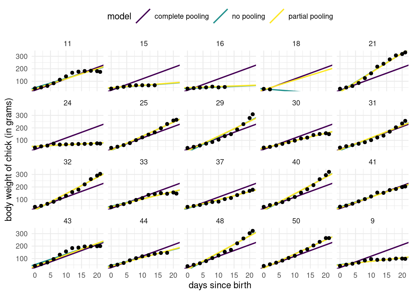
Figure 6.2: Partial pooling of coefficients for chicken data. Fitted regression lines for the model with a single common slope (complete pooling) and model with chick-specific intercept and slopes (no pooling). The conditional predictions are very close to individual slopes and barely distinguishable, except for chicken with fewer data points were they lie closer to the overall mean, one-size-fits-all model (i.e., complete pooling).

To better visualize this effect, we look at contour lines from the bivariate normal distribution of the random effects. This highlight the impact of having independent slope and intercept (circular contour curves for the bivariate normal distribution of the random effects). The arrows on Figure 6.3 illustrate this shrinkage effect: the points move towards region of higher density according to the random effect estimated density.

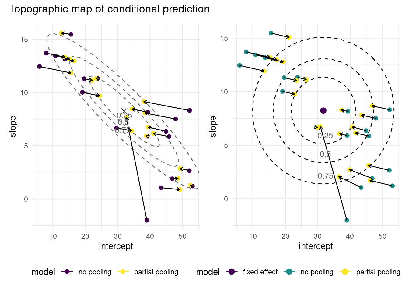
Figure 6.3: Graph of conditional predictions for the model with correlated (left) and independent (right) random effects on the intercept and slope of the chicken weight data. The conditional predictions, which include the predicted random effect specific to each chick, are shrunk towards the fixed effect, located in regions. The normal specification on the random errors induces a penalty for the estimates, which explains shrinkage. Adding correlation changes the shape of the penalty region (ellipsoidal rather than circular), thus inducing different constraints. Shorter series (fewer observations by chicken) are shrunk more towards the global estimated average.