4 Generalized linear models
Linear models are only suitable for data whose residuals are (approximately) normally distributed. However, there are many settings where we may wish to analyze a response variable which is not necessarily continuous, including when \(Y\) is binary, a count variable or is continuous, but non-negative. We will consider in particular likelihood-based inference for models of binary/proportion and counts data.
Generalized linear models (GLM) combine a model for the conditional mean with a distribution for the response variable and a link function tying predictors and parameters.
This chapter gives an introduction to generalized linear models and focuses in particular on logistic regression and Poisson regression, but only for the case of independent observations. Extensions of generalized linear models for correlated and longitudinal data, the so-called generalized linear mixed models (GLMM), are covered in MATH80621.
4.1 Basic principles
The starting point is the same as for linear regression: we have a random sample of independent observations \((\boldsymbol{Y}, \mathbf{X})\), where \(Y\) is the response variable and \(\mathrm{X}_1, \ldots, \mathrm{X}_p\) are \(p\) explanatory variables or covariates which are assumed fixed (non-random). The goal is to model the mean of the response variable as a function of the explanatory variables.
Let \(\mu_i=\mathsf{E}(Y_i \mid \mathbf{X}_i)\) denote the conditional expectation of \(Y_i\) given covariates and let \(\eta_i\) denote the linear combination of the covariates that will be used to model the response variable, \[\begin{align*} \eta_i=\beta_0 + \beta_1 \mathrm{X}_{i1} + \cdots + \beta_p \mathrm{X}_{ip}. \end{align*}\] The building blocks of the generalized linear model are
- A random component, consisting of the probability distribution for the outcome \(Y\) that is a member of the exponential dispersion family (normal, binomial, Poisson, gamma, \(\ldots\)).
- A deterministic component, the linear predictor \(\boldsymbol{\eta}=\mathbf{X} \boldsymbol{\beta}\), where \(\mathbf{X}\) is an \(n\times (p+1)\) matrix with columns \(\mathbf{1}_n, \mathbf{X}_1, \ldots, \mathbf{X}_p\) and \(\boldsymbol{\beta} \in \mathbb{R}^{p+1}\) are coefficients.
- A monotone function \(g\), called link function, that maps the mean of \(Y_i\) to the predictor variables, \(g(\mu_i)=\eta_i\).
4.2 Theory of generalized linear models
This section borrows from Chapter 4 of
Agresti (2015). Foundations of Linear and Generalized Linear Models, Wiley.
4.2.1 Exponential dispersion family of distributions
In a generalized linear model, the random component arises from an exponential dispersion family. Consider a probability density or mass function for \(Y\) with parameters \((\theta, \phi)\), \[\begin{align} f(y; \theta, \phi)&= \exp \left\{ \frac{y \theta -b(\theta)}{a(\phi)} + c(y, \phi)\right\}, \tag{4.1} \end{align}\] where the support, i.e., the set of values taken by \(Y\), doesn’t depend on the parameters. Throughout, we will assume the natural parameter \(\theta\) is unknown, but the dispersion parameter \(\phi\) may be known (exponential family) or unknown (exponential dispersion family).
One particularity of exponential dispersion models is that there exists an explicit relationship between mean and variance of \(Y\), which the following derivation shows. the first and second derivative of the log likelihood contribution of \(Y_i\), say \(\ell_i\), with respect to the natural parameter \(\theta\) are \[\begin{align*} \frac{\partial \ell_i(y; \theta, \phi)}{\partial \theta} &= \frac{\partial}{\partial \theta} \left\{\frac{y\theta-b(\theta)}{a(\phi)} + c(y, \phi) \right\} = \frac{y - b'(\theta)}{a(\phi)}\\ \frac{\partial^2 \ell_i(y; \theta, \phi)}{\partial \theta^2} &= - \frac{b''(\theta)}{a(\phi)}, \end{align*}\] where \(b'(\cdot)\) and \(b''(\cdot)\) are the first two derivatives of \(b(\cdot)\) with respect to \(\theta\). Under regularity condition, the Bartlett identities \[\begin{align*} \mathsf{E}\left\{\frac{\partial \ell(y; \theta, \phi)}{\partial \theta}\right\}=0, \qquad - \mathsf{E}\left\{\frac{\partial^2 \ell(y; \theta, \phi)}{\partial \theta^2}\right\} = \left[\mathsf{E}\left\{\frac{\partial \ell(y; \theta, \phi)}{\partial \theta}\right\}\right]^2. \end{align*}\] hold and these give \[\begin{align*} \mathsf{E}(Y_i) &= b'(\theta_i) \\ \mathsf{Va}(Y_i) &= b''(\theta_i)a(\phi_i) \end{align*}\] Often, the term \(a_i(\phi)=a_i\phi\), where \(\phi\) is constant over all observations and \(a_i\) is an observation-specific weight. The mean of \(Y_i\), say \(\mu_i\), and the natural parameter \(\theta_i\) are related through the equation \(\mu_i=b'(\theta_i)\). There is also an explicit relationship with the variance through \(V(\mu)=b''(\theta)\), unless \(V(\mu)=1\).
Example 4.1 (Poisson distribution as exponential family member) The mass function of the Poisson distribution is \[\begin{align*} f(y; \lambda) = \frac{\lambda^y \exp(-\lambda)}{y!} =\exp \left\{ y \ln (\lambda) -\lambda-\ln(y!)\right\}, \qquad y=0,1, \ldots \end{align*}\] The natural parameter is \(\theta =\ln(\lambda)\), the dispersion parameter \(\phi=1\), and \(b(\theta)=\exp(\theta)\). Replacing these expressions in the mean-variance formulas, we get \(\mathsf{E}(Y)=\exp(\theta)=\mu\) and \(\mathsf{Va}(Y)=\exp(\theta)=\mu\), meaning \(V(\mu)=\mu\).
Example 4.2 (Binomial distribution as member of the exponential family) We consider the mass function of a binomial distribution, \(\mathsf{Bin}(m, \pi)\), with the number of trials \(m\) known. The parametrization presented in Example A.3 is not convenient because the mean and the variance both depend on \(m\). We consider thus a different parametrization in which \(Y\) represents the proportion of successes, so the mass function takes values in \(\{0, 1/m, \ldots, 1\}\) and \(mY\) denotes the number of successes. The mass function for \(Y\) is then \[\begin{align*} f(y, \pi)&=\exp \left\{ my \ln \left( \frac{\pi}{1-\pi} \right) + m \ln (1-\pi) + \ln \left[ \binom{m}{my}\right]\right\}\\& =\exp \left\{ \frac{y \ln \left( \frac{\pi}{1-\pi} \right) + \ln (1-\pi)}{1/m}+ \ln \left[ \binom{m}{my}\right]\right\} \end{align*}\] Set \[\begin{align*} \theta= \ln \left( \frac{\pi}{1-\pi}\right) \end{align*}\] with \(b(\theta) = \ln\{1+\exp(\theta)\}\) and \(\phi=m^{-1}\). The expectation and variance are easily derived and \[\begin{align*} \mathsf{E}(Y)&=\pi = \mathrm{expit}(\theta)=\frac{\exp(\theta)}{1+\exp(\theta)}=\mu \\\mathsf{Va}(Y) &= \frac{\pi(1-\pi)}{m} = \frac{\mu(1-\mu)}{m} = \phi V(\mu) \end{align*}\] where \(V(\mu)=\mu(1-\mu)\).
Example 4.3 (Normal distribution as member of the exponential family) We consider a sample consisting of independent normal observations, \(Y_i \sim \mathsf{No}(\mu_i, \sigma^2)\), with \[\begin{align*} f(y_i, \mu_i, \sigma^2)&= (2\pi\sigma^2)^{-1/2} \exp \left\{ -\frac{(y_i-\mu_i)}{2\sigma^2}\right\} \\&= \exp \left[ \frac{y\mu - \mu^2/2}{\sigma^2} - \frac{1}{2} \left\{ \frac{y^2}{\sigma^2} + \ln(2\pi\sigma^2)\right\} \right], \end{align*}\] meaning \(\theta=\mu\), \(\phi=\sigma^2\) and \(a(\phi)=\sigma^2\), \(b(\theta)=\theta^2/2\).
4.2.2 Link functions
The link between the mean of \(Y\) and the linear predictor \(\eta\) is \[\begin{align*} g\left\{\mathsf{E}(Y \mid \mathrm{X}_1, \ldots, \mathrm{X}_p)\right\}=\eta = \beta_0 + \beta_1 \mathrm{X}_{1} + \cdots + \beta_p \mathrm{X}_{p}. \end{align*}\] The link function thus connects the mean of the random variable \(Y\) to the explanatory variables, \(g(\mu_i) = \eta_i = \beta_0 + \sum_{j=1}^p\beta_j\mathrm{X}_{ij}\) and likewise \(\mu_i = g^{-1}(\eta_i)\). If the link function is chosen such that \(\theta=\eta\), the link function is termed the canonical link function.
The need for a link function often arises from parameter constraints: for example, the mean \(\mu=\pi\) of a Bernoulli distribution is the proportion of successes and must lie in the interval \((0, 1)\). Similarly, the mean \(\mu\) of the Poisson distribution must be positive. For the normal distribution (ordinary linear regression model), the mean is unconstrained and the canonical link function is the identity, \(\mu_i = \eta_i\).
An appropriate choice of link function \(g\) sets \(\mu_i\) equal to a
transformation of the linear combination \(\eta_i\) so as to avoid
imposing parameter constraints on \(\boldsymbol{\beta}\). Certain choices
of link functions facilitate interpretation or make the likelihood
function convenient for optimization.
For the Bernoulli and binomial distributions, the most common link
function \(g\) is the logit function,
\[\begin{align*}
\mathrm{logit}(\mu)&=
\ln \left( \frac{\mu}{1-\mu} \right) =\ln(\mu) - \ln(1-\mu)= \eta,
\\\mathrm{expit}(\eta)&= \frac{\exp(\eta)}{1+\exp(\eta)}=\mu.
\end{align*}\]
The inverse link function is the distribution function of
the logistic distribution, hence the name logistic regression. This
choice of link function is far from unique: any quantile function of a
continuous random variable supported on \(\mathbb{R}\) could be
considered. For the Poisson distribution, the canonical link function
\(g\) is the natural logarithm, \(\ln\), with associated inverse link
function \(\exp\).
Canonical link functions are natural choices because of their nice statistical properties: choosing the canonical link ensures that \(\mathbf{X}^\top\boldsymbol{y}\) is a minimal sufficient statistic. Other considerations, such as parameter constraints, can be more important in deciding on the choice of \(g\).
Example 4.4 (Transforming a nonlinear regression model into a linear model through a link function) Consider a linear model for which theory dictates that the mean should be \(Y \sim \mathsf{No}\{\alpha_0/(1+\alpha_1x), \sigma^2\}\).
This model is nonlinear in \(\alpha_0\), \(\alpha_1\). If we opt for the reciprocal link function \(g(x)=1/x\), we get \(\beta_0+\beta_1 x\), where \(\beta_0 = 1/\alpha_0\) and \(\beta_1 = \alpha_1/\alpha_0\) provided \(\alpha_0 \neq 0\). Since the generalized linear model is estimated using maximum likelihood and the latter are invariant to reparametrization, we get easily the estimated coefficients of interest.
4.2.3 Likelihood inference for generalized linear models
Likelihood inference is straightforward, although some care is needed because the asymptotic distribution of test statistics sometimes depend on the model parameters. Under regularity conditions, the maximum likelihood estimators of \(\boldsymbol{\beta}\) and \(\phi\) are jointly normally distributed, \[\begin{align*} \widehat{\boldsymbol{\beta}} \stackrel{\cdot}{\sim}\mathsf{No}_{p+1}\{\boldsymbol{\beta}, (\mathbf{X}^\top\mathbf{W}\mathbf{X})^{-1}\} \end{align*}\] where \[\mathbf{W} = \mathrm{diag}\{w_1,\ldots, w_n\}, \qquad w_i = \frac{\left(\partial \mu_i/\partial \eta_i\right)^2}{\mathsf{Va}(Y_i)}=\{g'(\mu_i)^2a_i(\phi)V(\mu_i)\}^{-1}. \]
Since \(\mathbf{W}\) depends on the unknown \(\boldsymbol{\beta}\) through the expected values \(\mu_i\), we can estimate \(\widehat{\mathbf{W}}\) by replacing the unknown coefficients by their maximum likelihood estimates at \(\widehat{\boldsymbol{\beta}}\).
Example 4.5 (Elements of the weight matrix for Poisson data) If we consider \(Y_i \sim \mathsf{Po}(\mu_i)\) with canonical link function \(\mu_i = \exp(\eta_i)\), then \(\partial \mu_i/\partial \eta_i =\exp(\eta_i)= \mu_i\) and thus \(w_i=\mu_i\).
Since we use maximum likelihood estimation, the theory presented in Chapter 3 readily applies. For example, if we want to compare two nested models and test if \(q\) of the \(\boldsymbol{\beta}\) are jointly zero (corresponding to no effect for the associated covariates), we can fit both null and restricted models and perform a likelihood ratio test. Under regularity conditions, the likelihood ratio statistic to compare two nested models will follow the usual \(\chi^2_q\) distribution.
4.2.4 Goodness-of-fit criteria
Goodness-of-fit diagnostics often rely on test statistics comparing the fitted model with parameters \(\widehat{\boldsymbol{\beta}}\) with a saturated model in which there are \(n\) parameters for the mean, as many as there are observations — this amounts to maximizing the log-likelihood contribution of each term \(\ell_i\) individually, for which the best value of the linear predictor is denoted \(\widetilde{\eta}_i\) (oftentimes, this is when \(\widetilde{\mu}_i=y_i\)). We can then build a likelihood ratio statistic to compare the saturated model with the fitted model, taking \[\begin{align*} \frac{D}{\phi}= \sum_{i=1}^n 2\{\ell(\widetilde{\eta}_i; y_i) - \ell(\widehat{\eta}_i; y_i)\}. \end{align*}\] The scaled deviance \(D\) will be small when the quality of the adjustment is roughly the same for both models, whereas large values of \(D\) are indicative of poor fit.
Example 4.6 (Deviance for common generalized linear models) Suppose that the model matrix of the model \(\mathbf{X}\) includes an intercept and let \(\widehat{\mu}_i\) denote the fitted mean. Then, the deviance for the normal generalized linear model with homoscedastic errors is \(D = \sum_{i=1}^n (y_i - \widehat{\mu}_i)^2\), which is the sum of squared residuals. For Poisson data, the saturated model has \(\widetilde{\mu}_i=y_i\) and \(D= 2\sum_{i=1}^n y_i \ln(y_i/\widehat{\mu}_i)\).
Another alternative is found by looking at score test statistic comparing the saturated model with the postulated model with \(p+1\) parameters \(\boldsymbol{\beta}\). The Pearson \(X^2\) statistic is \[\begin{align*} X^2= \sum_{i=1}^n \frac{(y_i-\widehat{\mu}_i)}{ V(\widehat{\mu}_i)}, \end{align*}\] where both expectation and variance are estimated using the model; for Poisson data, \(\phi=1\) and the estimated mean and variance are equal, meaning \(\widehat{\mu}_i=V(\widehat{\mu}_i)\). Pearson’s \(X^2\) statistic measures standardized departures between observations and fitted values.
In large samples, both Pearson \(X^2/\phi\) and the deviance \(D/\phi\) follow approximately a \(\chi^2_{n-p-1}\) distribution if the model is correct and \(\phi\) is known (but this result doesn’t hold for binary data or binomial data unless \(m\) is very large and \(\boldsymbol{\beta}\) are small). If \(\phi\) is unknown, we would replace it throughout by an estimate and the same distributional results hold approximatively.
4.3 Binary responses
Binary response data are commonplace, notably due to their role in classification. We begin this section by discussing interpretation of the model in terms of censored observations, than tackle the interpretation of the parameters for the canonical link function on different scales (probability, odds and log-odds). We pursue with issues due to the nature of the data, including non-regular asymptotics and separation of variable.
The logistic model specifies \[\begin{align*} \mathsf{P}(Y_i=1 \mid \mathbf{X}_i) = \pi_i = \frac{\exp(\beta_0 + \beta_1 \mathrm{X}_{i1}+ \cdots + \beta_p\mathrm{X}_{ip})}{1 + \exp(\beta_0 + \beta_1 \mathrm{X}_{i1}+ \cdots + \beta_p\mathrm{X}_{ip})}, \end{align*}\] whereas, on the linear predictor scale \(\eta_i\), \[\begin{align*} \eta_i =\log \left(\frac{\pi_i}{1-\pi_i}\right) = \beta_0 + \beta_1 \mathrm{X}_{i1}+ \cdots + \beta_p\mathrm{X}_{ip}. \end{align*}\]
One way to view binary variables is as censored observations: suppose \(Z_i = \eta_i + \varepsilon_i\) where \(\varepsilon_i\) is an error term with distribution function \(F\) and \(\eta_i\) is a fixed linear predictor. Suppose that the variables \(Z_i\) are censored:we only observe the binary indicators \(Y_i = 1\) if \(Z_i > 0\) and \(Y_i=0\) otherwise, not the \(Z_i\) terms themselves. It follows that \[ \mathsf{P}(Y_i = 1 \mid \eta_i) = 1-F(-\eta_i) \] If \(F\) is symmetric around zero, then \(F(\eta_i) = 1-F(-\eta_i)\). The choice of the logistic distribution for \(F\) gives \(\pi_i = \mathrm{expit}(\eta_i)\). Another popular alternative is when \(F\) is the distribution function of a standard normal distribution, \(F(x) = \Phi(x)\), which is the probit regression model. Both link functions only differ in the tail, but the parameters of the the logistic model are more readily interpreted since the quantile function \(F^{-1}\) of the logistic distribution, \(\mathrm{logit}(x)\), is available in closed-form.
Dichotomization leads to a loss of information relative to the underlying continuous data, which translates into more variability in the parameter estimates.
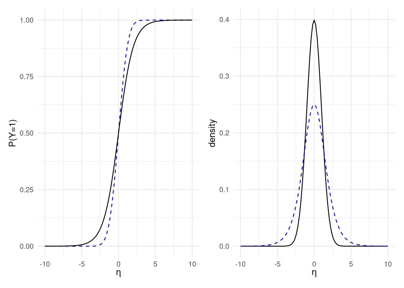
Figure 4.1: Comparison of logistic (black) and probit (dashed blue) inverse link functions (left) for binary data: both are monotone increasing functions of the linear predictor. The logistic distribution has thicker tails and thus smaller peak at zero. The right panel shows the derivative of both inverse link functions.
The logistic regression model is nonlinear in \(\boldsymbol{\eta}=\mathbf{X}\boldsymbol{\beta}\) and the left panel of Figure 4.1 shows how changes in the linear predictor impact the probability of success. As \(\eta_i\) increases (for example, if \(\mathrm{X}_j\) increases by one unit and \(\beta_j\) is positive), so does the estimated probability of success because the function \(\mathrm{expit}(x)\) is monotone increasing. This characterization is however not helpful. If we exponentiate the linear predictor \(\eta\), we get \[\begin{align*} \mathrm{odds}(Y\mid \mathbf{X}) = \frac{\pi(\mathbf{X})}{1-\pi(\mathbf{X})}=\exp(\beta_0+ \beta_1 \mathrm{X}_1 + \cdots + \beta_p\mathrm{X}_p), \end{align*}\] where \(\pi(\mathbf{X})/\{1-\pi(\mathbf{X})\}\) are the odds of \(\mathsf{P}(Y=1 \mid \mathbf{X})\) (success) relative to \(\mathsf{P}(Y=0 \mid\mathbf{X})\) (failure). If \(\pi=0.8\), the odds are \(\pi/(1-\pi)=0.8/0.2=4\): on average, we expect four successes for one failure.
On the odds scale, the logistic regression model is multiplicative: for an increase of \(\mathrm{X}_j\) of one unit, ceteris paribus, the odds are multiplied by \(\exp(\beta_j)\).
Example 4.7 (GPA score and graduate admission) We consider a simple logistic model for graduate admission (yes/no) in universities across the USA as a function of their grade point average (GPA).
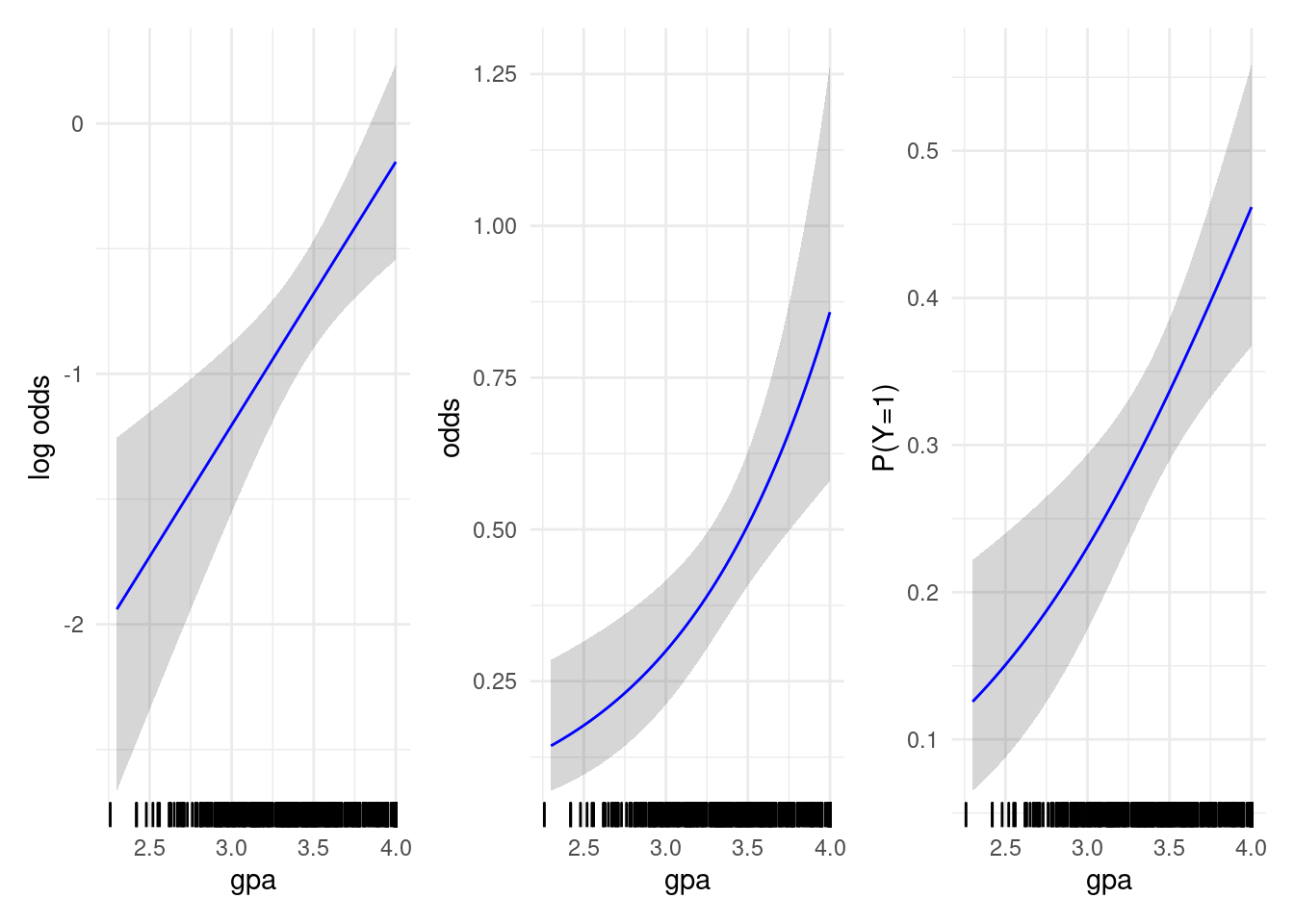
Figure 4.2: Graduate admission probability as a function of grade point averages (GPA) on the log odds (left), odds (middle) and probability of success scale (right). The line indicates fitted value with pointwise 95% profile-based confidence intervals.
| term | estimate | std. error | Wald stat. | p-value |
|---|---|---|---|---|
| (Intercept) | -4.36 | 1.04 | -4.21 | < 0.001 |
| gpa | 1.05 | 0.3 | 3.52 | < 0.001 |
The coefficients of the simple logistic model are reported in Table 4.1, showing that the log odds of admission increase by 0.11 for each increase in GPA of \(0.1\). This translates into \(\exp(0.1\widehat{\beta}_{\mathrm{gpa}})=1.11\) on the odds ratio scale, meaning a 11% increase in odds of admission for every \(0.1\) increase in GPA. Of course, this model is simplistic and omits other important factors\(\ldots\) Figure 4.2 shows the variation on the log odds, odds and probability scale as a function of grade point average. While the probability scale is the most intuitive, the effect of an increase of \(0.1\) unit of GPA isn’t the same, depending on what is your starting value: according to the model, the absolute increase in the probability of admission for individuals with GPA scores \(2.3\) and \(2.4\) is 1.2%, whereas that corresponding to an increase in GPA from 3.9 to 4 is 2.6%; this illustrates how the impact of an increase of \(0.1\) points is not the same across the board.
Example 4.8 (Risk factors related to underweight babies at birth) We consider a medical example related to risk factors explaining the birth weight: the birth weight is dichotomized and classified as low if the infant weight is inferior to 2.5 kg (1) and 0 otherwise. The data were collected in a medical center in Massachusetts in 1986.
The data contains the following explanatory variables
age: mother’s age in years.lwt: mother’s weight in pounds at last menstrual period.race: mother’s race (white,blackorother).smoke: smoking status during pregnancy (yes/no).ptl: previous premature labours (none/at least one).ht: history of hypertension.ui: presence of uterine irritability.
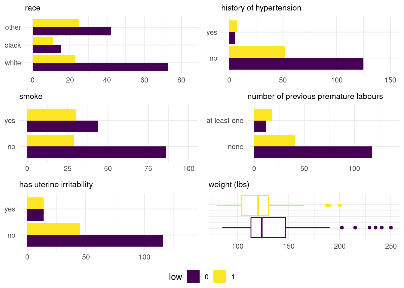
Figure 4.3: Exploratory data analysis for the birthweight data
The exploratory data analysis suggests that smoking has a large impact, as the relative proportion of women who smoke having underweight babies is significant. Likewise, hypertension seems to bean important predictor but there are only a handful of women in the sample with this condition. Women who previously gave birth to premature babies are more likely to give birth to underweight (and potentially premature) babies, whereas women giving birth to babies under 2.5kg also typically have lower weight. We can use a logistic regression to assess the effect of these explanatories.
| term | estimate | std. error | Wald stat. | p-value |
|---|---|---|---|---|
| (Intercept) | -0.13 | 0.97 | -0.13 | 0.9 |
| mother’s weight (lbs) | -0.02 | 0.01 | -2.29 | 0.022 |
| race [black] | 1.3 | 0.53 | 2.46 | 0.014 |
| race [other] | 0.85 | 0.44 | 1.94 | 0.053 |
| smoker [yes] | 0.87 | 0.4 | 2.14 | 0.032 |
| previous premature labours | 1.13 | 0.45 | 2.51 | 0.012 |
| hypertension [yes] | 1.87 | 0.71 | 2.64 | 0.008 |
| uterine irritability | 0.75 | 0.46 | 1.64 | 0.1 |
Table 4.2 gives the estimated coefficients \(\widehat{\boldsymbol{\beta}}\) on the logs odds scale along with standard errors, Wald statistics and the \(p\)-values from the normal approximation.
We can interpret the effect of these variables: given the other variables and ceteris paribus:
- the odds of giving birth to an underweight babies decrease by 1.6% for each additional pound pre-pregnancy; this paradoxical interpretation, at odds with Figure 4.3 is (notably) due to the correlation between smoking and mother’s weight.
- the odds of black women giving birth to an underweight baby are 2.67 times those of white women.
- the odds of women who smoke of having a baby weighting less than 2.5kg at birth are 137.9% higher than those of women who do not smoke.
The other parameters are interpreted accordingly. We can also check the parameter significance, by comparing the model with all the covariates and withholding one of the explanatories at the time. The results of the likelihood ratio test are presented in Table 4.3. At level 5% and given the other factors, having previous premature labours history and uterine irritability are not statistically significant. There is no significant correlation between the explanatories, since all the variance inflation factors are inferior to \(1.5\).
| variable | lik. ratio | df | p-value |
|---|---|---|---|
| mother’s weight | 5.96 | 1 | 0.015 |
| race | 7.61 | 2 | 0.022 |
| smoker | 4.72 | 1 | 0.03 |
| previous premature labours | 6.37 | 1 | 0.012 |
| hypertension | 7.31 | 1 | 0.007 |
| uterine irritability | 2.63 | 1 | 0.1 |
4.3.1 Issues with binary data
One oddity of regression models for binary data is that most of the information in the sample is provided by response whose variance is largest (points that have \(\pi\) far from 0 or 1). This can be seen by looking at how the probability \(\pi\) changes as a function of changes in the \(j\)th explanatory \(\mathrm{X}_j\): if \(\pi = \mathrm{expit}(\beta_0 + \beta_1\mathrm{X}_1 + \cdots + \beta_p\mathrm{X}_p)\), then \(\partial \pi/\partial \mathrm{X}_j = \beta_j \pi(1-\pi)\), so the effect of \(\beta_j\) is large when \(\pi\) is near \(0.5\) and near zero if the probabilities are close to the endpoints \(0\) or \(1\). Thus, if one wants to estimate a coefficient \(\beta_j\) of large magnitude, the ratio \(|\beta_j|/\mathsf{sd}(\beta_j) \to 0\) as \(\beta_j \to \infty\): the power for testing that \(\beta_j=0\) using a Wald statistic tends to zero. Wald statistics are not recommended for Bernoulli data: the following simple example illustrates why.
Example 4.9 (Incoherent results for Wald tests) Suppose we consider a simple binary model and \(n=100\) observations and the null hypothesis \(\mathscr{H}_0:\pi = 0.5\) and equivalently for the logistic model \(Y_i \sim \mathsf{Bin}\{m, \mathrm{expit}(\beta_0)\}\), where this same hypothesis amounts to \(\mathscr{H}_0:\beta_0=0\). Figure 4.4 clearly shows that lack of invariance of the Wald statistic to reparametrization. When \(\widehat{\beta}_0\) increases and \(m\) is large, the Wald statistic for \(\beta_0\) decreases as we approach \(m\) successes, because the standard error of \(\widehat{\beta}_0\) increases faster than the difference \(\widehat{\beta}-0\). Both statistics are asymptotically normal if the null hypothesis holds true, so the two-sided test would reject if the value of the Wald statistic is greater than 1.96. Depending on the parametrization, however, they give different results: the statistic increases monotonically for \(\pi\), but would converge to zero for \(\beta_0\) when \(m\) is large (allowing thereby larger values of \(\widehat{\beta}_0\)). No such problem arises when considering score and likelihood ratio tests.
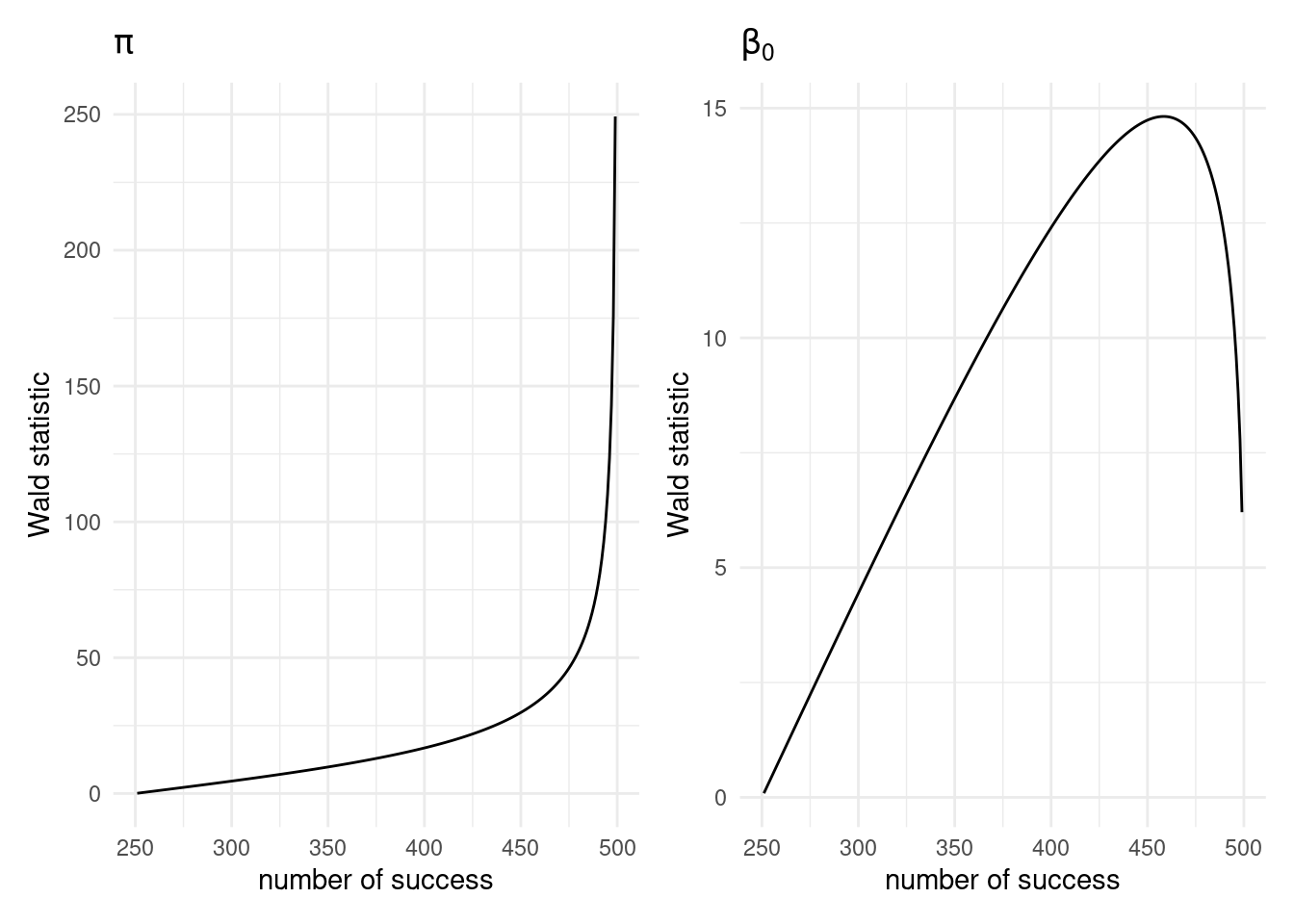
Figure 4.4: Wald test statistic for \(Y_i \sim \mathsf{Bin}(m=500, \pi)\) (left) for \(\pi=0.5\) and the same hypothesis test on the logistic scale with \(Y_i \sim \mathsf{Bin}(m=500, \mathrm{expit}(\beta_0))\) and \(\mathscr{H}_0:\beta_0=0\) (right) as a function of the number of success out of 500 trials.
Thus, information about the coefficients only accumulates if the true regression coefficients \(\boldsymbol{\beta}\) are small. The deviance and Pearson provide little to no information about the quality of the model adjustment and their null distribution depends on \(\widehat{\boldsymbol{\beta}}\): with large coefficients, the asymptotic \(\chi^2\) distribution is not a good approximation and relying on these to determine goodness-of-fit is not recommended.
4.3.2 Quasi-separation of variables
One common problem with binary data is the problem of complete separation of variables: in this scenario, a linear combination of the explanatories allows to perfectly categorize \(Y_i\) into \(0/1\) depending on the value of the covariates and the predicted probabilities will be exactly zero or one. While this is not a problem for prediction, the coefficients that yield such a sharp transition are near infinite, as displayed in Figure 4.5; software may or not pick up such error, but in any case Wald tests for individual coefficients are rubbish. This is problematic for inference because we cannot meaningfully interpret the resulting parameters.
|
|
Inspection of the coefficients and their standard errors is a good way to detect such problems: parameters that are large (with standardized explanatories with mean zero variance one inputs) with \(|\widehat{\beta}_j| > 36\) are particularly suspicious; the number of iterations for the optimization routine is also often abnormally large. While the Wald statistic for \(\beta_1=0\) is nearly zero and the \(p\)-value 1, the likelihood ratio test yields a statistic of \(20.016\) with a negligible associated \(p\)-value.
One way to restore finiteness of the \(\boldsymbol{\beta}\) is to impose a penalty term that prevents near infinite parameter values. Firth’s penalty is the most popular solution (option firth in the SAS procedure logistic and logistf::logistf function in R.
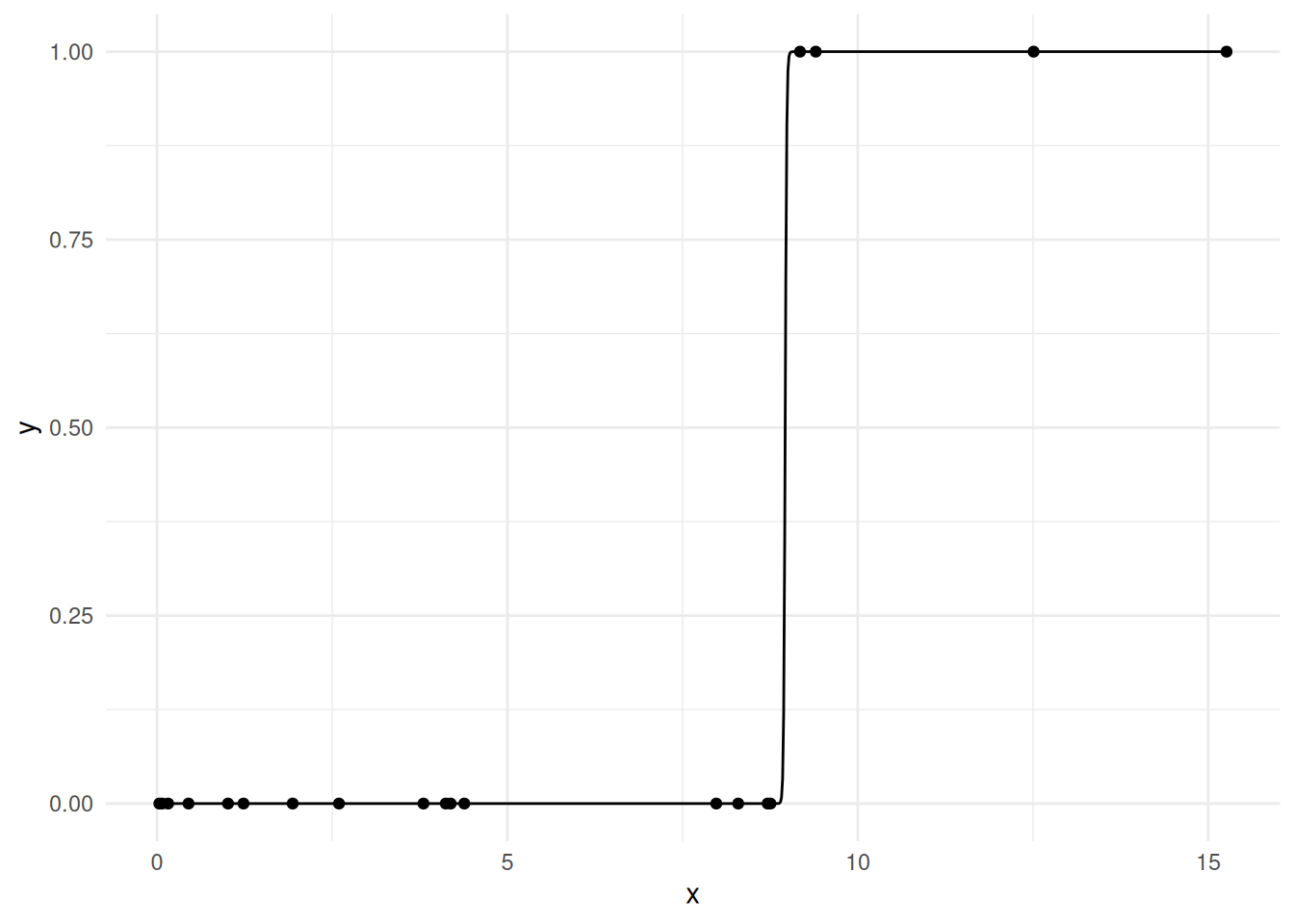
Figure 4.5: Illustration of complete separation of variable on simulated observations. Parameters are near infinite to yield a sharp transition at \(x=9\). Quasi-complete separation of variable occurs if both outcomes are observed at the cutoff point.
4.4 Count data
If a response is integer value, the linear model is seldom appropriate because the variable is skewed, which even the log-linear model may fail to capture. It may thus be appropriate to look at generalized linear models for discrete data.
The most widespread model for count data is the Poisson regression. The Poisson distribution arises as the limit of binomial data with a small probability of success as the number of attempts becomes large: examples include rare medical conditions, number of accidents, or goals in a soccer (football) match. The mean and variance of the Poisson distribution are both \(\lambda\), so the model imposes stringent constraints on the observations. Extensions that deal with zero-inflation, underdispersed and overdispersed data are widespread.
The canonical link of the Poisson model is the natural logarithm \(\ln(x)\) and the interpretation will be similar to that of the log-linear model. Specifically, suppose the mean model is \[\begin{align*} \mu = \exp(\beta_0 + \beta_1 \mathrm{X}_{1} + \cdots + \beta_p \mathrm{X}_{p}), \end{align*}\] so the mean is multiplied by \(\exp(\beta_j)\) for an increase of one unit of \(\mathrm{X}_{j}\), ceteris paribus. If \(\beta_j < 0\), \(\exp(\beta_j) < 1\) and so we have a decrease of \(100\cdot(1-\exp(\beta_j))\)% of the mean response. Likewise, if \(\beta_j>0\), the mean number increases by \(100\cdot(\exp(\beta_j)-1)\)%. The interpretation of interactions between categorical and continuous/categorical variables is similar to that of multiplicative (log-linear) models.
Example 4.10 (Road accidents and speed limits on the motorway in Sweden) Sweden is a worlwide leader in road safety and has a long history of countermeasures to increase road traffic safety, including the Vision Zero program. Back in the 1960s, a study was conducted by the authorities to investigate the potential of speed limits on motorways to reduce the number of accidents. The sweden data contains the number of accidents on 92 matching days in both 1961 and 1962 (Svensson 1981); speed limits were in place on selected days in either year.
We consider an example from Section 4.5 of Brazzale, Davison, and Reid (2007). To study the impact of the restrictions we can fit a Poisson model. Let \(Y_{i1}\) (respectively \(Y_{i2}\)) denote the number of accidents in 1961 (1962) on day \(i\) and let \(\texttt{limit}_{ij}\) denote a binary indicator equal to one if speed limits were enforced on day \(i\) of year \(j\). We set \[\begin{align*} Y_{i1} \sim \mathsf{Po}(\delta_i + \alpha \texttt{limit}_{i1}), \quad Y_{i2} \sim\mathsf{Po}(\delta_i + \gamma + \alpha \texttt{limit}_{i2}), \qquad i=1, \ldots, 92. \end{align*}\] The nuisance parameters \(\delta_1, \ldots, \delta_{92}\) control for changes in background number of accidents and are of no practical interest, while \(\gamma\) denotes the change from 1961 to 1962. We are interested here in assessing changes in the number of accidents due to the policy, \(\alpha\); of secondary interest is to determine whether there has been a decrease in the number of accident relative to 1961.
| variable | lik. ratio | df | p-value |
|---|---|---|---|
| day | 9395.22 | 92 | < 0.001 |
| limit | 46.29 | 1 | < 0.001 |
| year | 0.7 | 1 | 0.4 |
The residual deviance is 107.95 for 90 degrees of freedom, suggests the overall fit is good, despite the large number of nuisance parameters \(\delta_1, \ldots, \delta_{92}\). The coefficient associated to limit is strongly significant: the estimated coefficient is \(\widehat{\alpha}=-0.292\), indicates that speed limits reduce the mean number of accidents by \(25.3\)% on average. In contrast, the likelihood ratio test reported in Table 4.5 shows that the change in the yearly number of accident from 1961 to 1962, \(\gamma\), is not significantly different from zero.
4.4.1 Overdispersion
One restriction of the Poisson model is that the restriction on its moments is often unrealistic. We tackle the problem of overdispersion, for which the variability in the counts is larger than that implied by a Poisson distribution.
Overdispersion is not the only problem encountered in practice: sometimes, the variance is smaller than the mean, typically due to excess of zeros. Hurdle models and zero-inflated models can be used to deal with this issue. The most common framework for handling overdispersion is to consider that the mean \(\lambda\) of the Poisson distribution is itself a positive random variable with mean \(\mu\). By the laws of iterated expectation and iterative variance, \[\begin{align*} \mathsf{E}(Y) &= \mathsf{E}_{\Lambda}\{\mathsf{E}(Y \mid \Lambda\} = \mathsf{E}(\Lambda) = \mu\\ \mathsf{Va}(Y) &= \mathsf{E}_{\Lambda}\{\mathsf{Va}(Y \mid \Lambda)\} + \mathsf{Va}_{\Lambda}\{\mathsf{E}(Y \mid \Lambda)\} = \mathsf{E}(\Lambda) + \mathsf{Va}(\Lambda) = \mu + \mathsf{Va}(\Lambda). \end{align*}\] This hierarchical model thus necessarily yield a model in which the variance is higher than the mean. If \(\Lambda\) follows a gamma distribution with scale \(k\mu\) and rate \(k>0\), \(\Lambda \sim \mathsf{Ga}(k\mu, k)\), the marginal distribution for the response \(Y\) follows a negative binomial distribution, whose mean and variance are \[\begin{align*} \mathsf{E}(Y) = \mu, \qquad \mathsf{Va}(Y) = \mu + k \mu^2. \end{align*}\] The term \(k\) is a dispersion parameter, which is fixed for all observations. As \(k \to 0\), the distribution of \(\Lambda\) degenerates to a constant at \(\mu\) and we recover the Poisson model. While both negative binomial and Poisson models are nested, the likelihood ratio test is non-regular because the restriction we test lies on the boundary of the parameter space, as \(k \in (0, \infty)\). The consequence is that, in large samples, if the data are truly Poisson and we fit a negative binomial, we expect the maximum likelihood estimator of the dispersion parameter \(k\) to be exactly zero half of the time and to be positive and behave like a \(\chi_1^2\) random variable the other half of the time.
Strictly speaking, the negative binomial expansion presented above is not a generalized linear model unless \(k\) is known, but we can write down the log-likelihood and fit the model by alternating maximization of \(\boldsymbol{\beta}\) and \(k\) and perform likelihood-based inference as usual.
Example 4.11 We can ascertain the finite sample properties of the likelihood ratio test by simulating repeatedly from a Poisson regression model, fitting the negative binomial model and calculating the likelihood ratio statistic. Since the negative binomial model yields \(k>0\), we include \(k=0\) by fitting a Poisson model and keeping the latter whenever it yields a higher log likelihood than the one found by maximizing the negative binomial model.
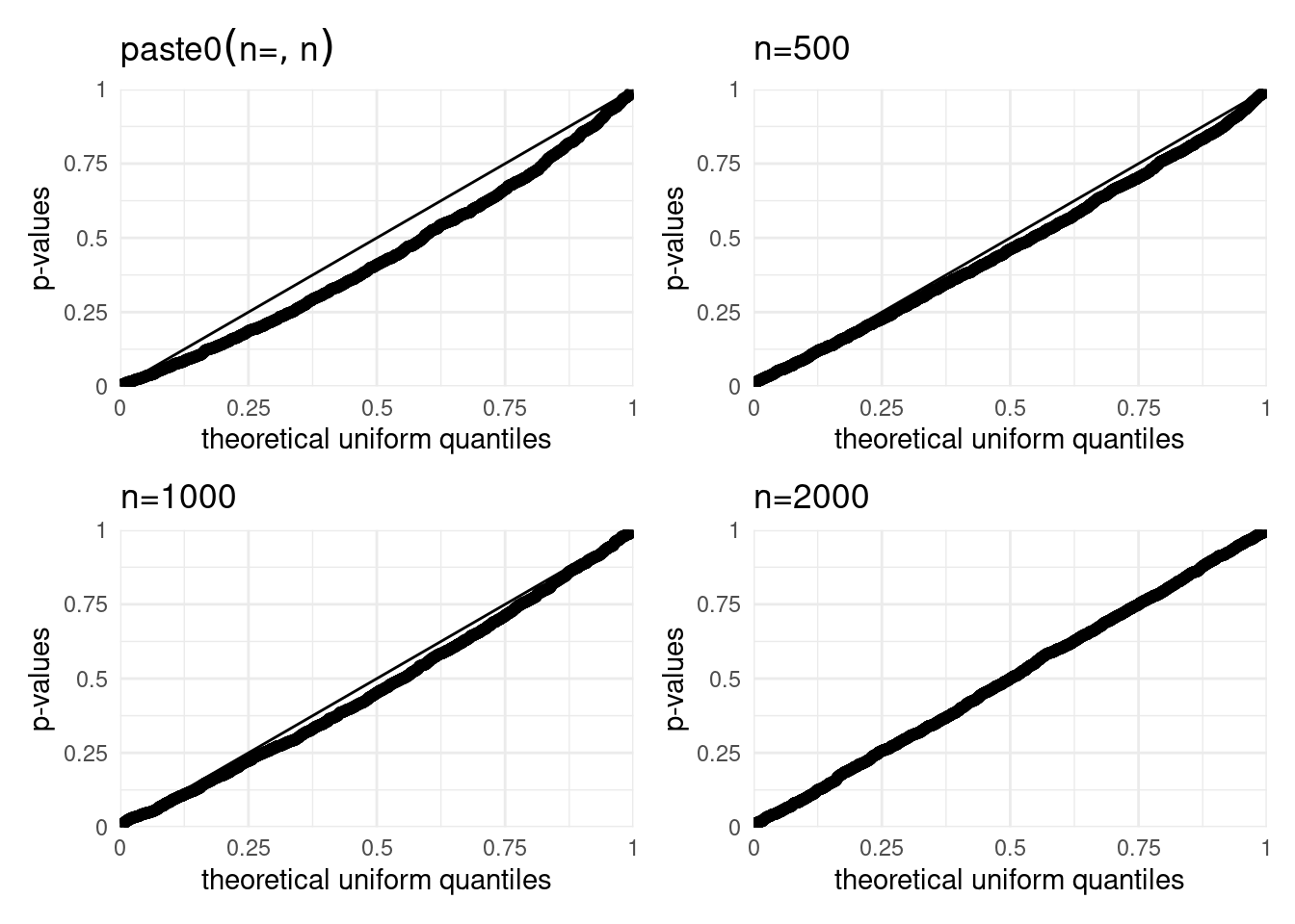
Figure 4.6: Simulated null distribution of the likelihood ratio test comparing the Poisson and negative binomial regression models. The quantile-quantile plot show the distribution of positive statistics for sizes \(n=100, 500, 1000, 2000\) relative to the asymptotic \(\frac{1}{2}\chi^2_1\).
The percentage of likelihood ratio statistics that are zero is \(69\)%, \(60\)%, \(59\)% and \(54\)% for respectively \(n=100\), \(500\), \(1000\) and \(2000\). We can also see from the quantile-quantile plots that the empirical distribution of the positive values is right skewed relative to the \(\chi^2_1\) reference. This strongly suggest that asymptotic null distribution, consisting of a point mass with probability half at \(0\) and \(\chi^2_1\) with probability half is seemingly valid only for very large samples; bear in mind that these findings also don’t account for model misspecification.
4.4.2 Contingency tables
Most count data are found in contingency tables, in which the cells give the counts for each combination of factors and the dimensions of the table represent categorical variables. Such data format are convenient for storage and display, but must be transformed to long format for model fitting.
An \(m\) dimensional contingency table corresponds to a data frame with \(m\) categorical variables and the saturated model is the model with all main effects and all of the \(k\) (\(2 \leq k \leq m)\) interactions. The saturated model has as many coefficients as observations (here the product of the contingency table dimensions). Since the fitted value from this model are equal to the observed counts, it is unnecessary to fit the model: the likelihood ratio statistic for comparing the saturated model with a simpler alternative is simply the deviance statistic reported in the output, whereas the score test is given by Pearson \(X^2\) statistic. Inference proceeds as usual.
Example 4.12 (Poisson log-linear model for drug history in Dayton) We consider data from Agresti (2019) on history of high school students near Dayton, Ohio. A survey asked students from grade 12 about their previous consumption of alcohol, cigarettes and marijuana (yes/no). The \(2 \times 2 \times 2\) table corresponds to a 12 by 4 data frame with three binary variables and one integer-valued response giving the counts.
| marijuana | ||||||||
| alcohol | cigarette | no | yes | |||||
| no | no | 279 | 2 | |||||
| yes | 43 | 3 | ||||||
| yes | no | 456 | 44 | |||||
| yes | 538 | 911 | ||||||
With contingency tables, only categorical explanatory variables are available. The most complicated model, the saturated model with the three-way and all of two-way interactions, returns the observed counts. One can thus fit the model with all of the two-way interactions (with one parameter for the intercept, two for the main effects and three for the two-way interactions). Other models include selected two-way interactions and main effects.
| AM CM | AC CM | AC AM | AC AM CM | ACM |
|---|---|---|---|---|
| 909.2 | 885.9 | 710.0 | 910.4 | 911 |
| 438.8 | 563.1 | 739.0 | 538.6 | 538 |
| 45.8 | 29.4 | 245.0 | 44.6 | 44 |
| 555.2 | 470.6 | 255.0 | 455.4 | 456 |
| 4.8 | 28.1 | 0.7 | 3.6 | 3 |
| 142.2 | 17.9 | 45.3 | 42.4 | 43 |
| 0.2 | 16.6 | 4.3 | 1.4 | 2 |
| 179.8 | 264.4 | 276.7 | 279.6 | 279 |
We can test for restrictions from the saturated model. The likelihood ratio test statistic is the deviance statistic 0.37 whose value is far lower than the 0.95 quantile of the \(\chi^2_1\) distribution, \(3.84\). We thus fail to reject the null hypothesis \(\mathscr{H}_0:\beta_{\mathrm{ACM}}=0\), corresponding to no three-way interaction or equivalently to the hypothesis that the model with all two way interactions is an adequate simplification of the saturated model. Additional likelihood ratio tests reveal that further simplifications lead to significant decrease in goodness-of-fit. This is not surprising in light of the fitted value from each model, reported in Table 4.6: while the counts are not much off for the selected model, there is significant discrepancies between observed and predicted counts for the simpler alternatives.
4.5 Modelling proportions
Oftentimes, binary response are aggregated and we have access to a sample of \(n_i\) response with the same explanatory variables: we have multiple successes and failures observed for each combination of the covariates \(\mathbf{x}_i\). The response \(Y_i\) is the total number of success out of \(n_i\) trials, so \(Y_i \sim \mathsf{Bin}(n_i, \pi_i)\) where \(\pi_i = \mathrm{expit}(\mathbf{x}_i^\top\boldsymbol{\beta})\), say. Since the log likelihood of the Bernoulli distribution and that of the binomial are equal up to an additive constant factor, log likelihood and information criteria values will also differ by a constant factor, but the latter does not matter when making comparisons between models.
We can use a logistic model to estimate the probability of success; the only difference is that we need to provide the software with the number of success/failures or else success/trials. The data could also be un-grouped, then fitted using a Bernoulli model.
Example 4.13 (Smoking and the Grim Reaper) We consider survey data for a study conducted in 1972–1974 near Newcastle, UK. Information about smoking habits of women were collected; A follow-up of the same subjects was conducted 20 years later to evaluate how smoking habits affected survival. 162 women had smoked before 1972 but had stopped by 1972, and smoking habits were unknown for 18 women: these 180 women were excluded. The data consists of the remaining 1314 women. The smoker and non-smoker columns contain the number of dead/total (% dead).
Based on raw numbers, 582 women were smokers and 139 died (\(76.117\)% survival rate), whereas 230 of the of the 732 smokers died (\(68.6\)% survival rate). A logistic model for the number of survivors out of the total, based on smoking status, \[\mathsf{P}(\texttt{survive=yes} \mid \texttt{smoking}) = \mathrm{expit}(\beta_0+\beta_1 \mathsf{I}_{\texttt{smoking=yes}}), \] would return precisely these two probabilities of survival. The marginal odds of survival after twenty years are \(\exp(0.379) = 46\)% higher for smokers. It seems puzzling that smoking would lead to higher survival after twenty years and be effective at hiding from the Grim reaper, but this analysis omits an important fact: the smokers in the study were much younger than the non-smokers. In this situation, averaging over all age groups, a confounder, lead to an incorrect assessment of the effect of smoking since most non-smokers recruited were above the age of 64 and thus had lower survival probability of surviving 20 years to begin with. The breakdown of death is depicted in the mosaic plot of Figure 4.7. We see that more younger people were smoking, so the confounding effects leads unsurprisingly to smaller proportion of death in this group.
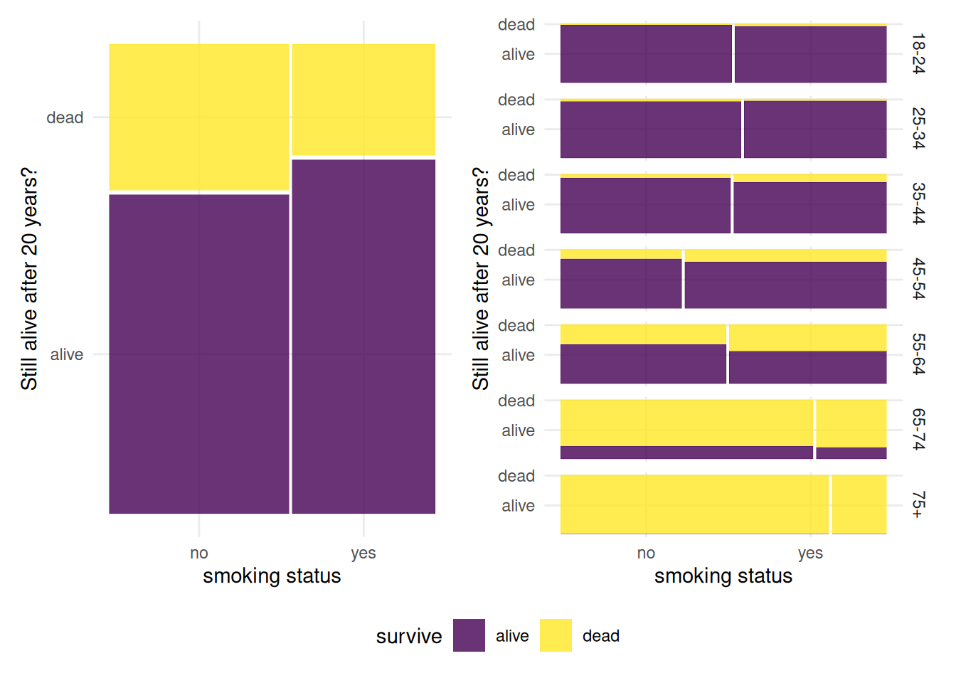
Figure 4.7: Mosaic plots for the smoker survival data: the left panel shows sample proportions of survivors depending on smoking status, whereas the right panel gives the sample proportion within each strata. Most of the people above 75 are non-smokers, and their probability of surviving beyond 95 years is small.
| coefficient | estimate | std. error |
|---|---|---|
| (Intercept) | 3.86 | 0.59 |
| smoker [yes] | -0.43 | 0.18 |
| age [25-34] | -0.12 | 0.69 |
| age [35-44] | -1.34 | 0.63 |
| age [45-54] | -2.11 | 0.61 |
| age [55-64] | -3.18 | 0.6 |
| age [65-74] | -5.09 | 0.62 |
| age [75+] | -27.81 | 11293.14 |
Table 4.7 gives the estimated coefficients of the logistic regression model for survival, where the baseline is survival for people aged 18-24; there is a steady decline in survival as age increases, with separation of variable for the last category (because everyone aged 75 and above were dead at follow-up). Age is strongly significant, leading to a likelihood ratio statistic of \(629.915\) for 6 degrees of freedom. The estimated effect of smoking is negative, so conditional on an age group, the estimated survival is multiplied by \(\exp(-0.427\)) with 95% likelihood ratio confidence intervals for this coefficient of [\(0.46\), \(0.92\)] on the odds scale. The point estimate corresponds to a \(34.8\)% decrease.
This phenomenon is termed Simpson’s paradox and is further illustrated in Figure 4.8: an incorrect marginalization over a confounder can lead to reverse effects, even when analysis withing subgroups leads to opposition conclusions for the effect of that variable.
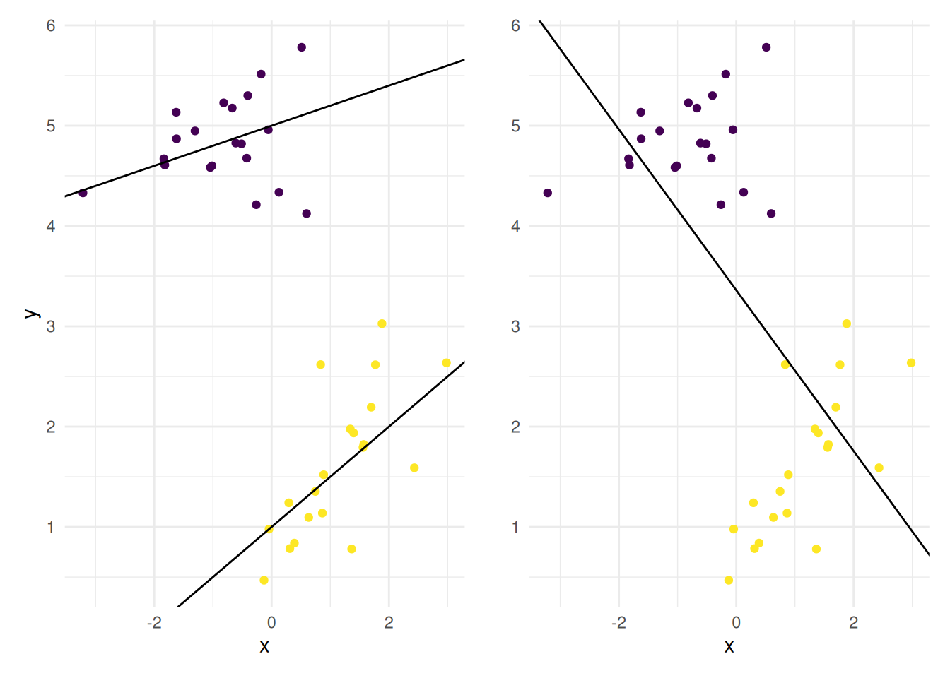
Figure 4.8: Illustration of the marginalization problem: within each subgroup, there is a clear positive correlation between explanatory and response, but averaging over all groups leads to incorrect estimates and a negative trend.
4.5.1 Conditional binomial likelihood for Poisson counts
Consider independent Poisson counts \(Y_1, Y_2\) with respective means \(\lambda_1, \lambda_2\). Suppose the total counts \(Y_1 + Y_2 = m\) and we condition on this quantity: the distribution of \(Y_2 \mid Y_1 + Y_2=m \sim \mathsf{Bin}\{m, \lambda_2/(\lambda_1 + \lambda_2)\}\). If we model each mean parameter as, \(\ln(\lambda_i) = \alpha + \mathbf{x}_i^\top\boldsymbol{\beta}\) where \(\mathbf{x}_i\) is a \(p\) row vector, then \[\begin{align*} \frac{\lambda_2}{\lambda_1 + \lambda_2} = \frac{\exp\{(\mathbf{x}_2-\mathbf{x}_1)^\top\boldsymbol{\beta}\}}{1+\exp\{(\mathbf{x}_2-\mathbf{x}_1)^\top\boldsymbol{\beta}\}}. \end{align*}\] We could thus estimate \(\boldsymbol{\beta}\) using a logistic regression, but the common intercept \(\alpha\) that appears in the mean of the Poisson counts is not estimable based on this conditional likelihood.
Example 4.14 Looking again at the data in Example 4.10, we condition on the sum of the number of accidents in 1961 and 1962, \(Y_{i1} + Y_{i2}\), and adjust the same mean model for the Poisson data.
Recall \[\begin{align*} \frac{\lambda_{i2}}{ \lambda_{i1} + \lambda_{i2}} &= \frac{\exp(\delta_i + \gamma + \alpha \texttt{limit}_{i2})}{(\exp(\delta_i + \gamma + \alpha \texttt{limit}_{i2}) + \exp(\delta_i + \alpha \texttt{limit}_{i1})} \\&= \frac{\exp\{\gamma + \alpha(\texttt{limit}_{i2}-\texttt{limit}_{i1})\}}{1+{\exp\{\gamma + \alpha(\texttt{limit}_{i2}-\texttt{limit}_{i1})\}}}, \qquad i=1, \ldots, 92. \end{align*}\]
In this case, we were not interested in the nuisance parameters \(\delta_1, \ldots, \delta_{92}\), which were there merely for the sake of controlling for daily changes. The binomial logistic model has only two parameters, but 92 observations rather than 184 since we regroup the counts. The parameter estimates (standard errors) based on the logistic regression are \(\widehat{\alpha} = -0.292 (0.043)\) and \(\widehat{\gamma}=-0.029(0.035)\), so enforcing a speed limit reduces the accident rate by \(\exp(-0.292)=0.75\), corresponding to a 25% decrease. The 95% profile likelihood confidence interval for this reduction, \(\exp(\alpha)\), is \([0.60, 0.81]\), and there are thus strong evidence that the reduction in the number of accident is real. The confidence interval for \(\gamma\), on the other hand, is \([-0.097, 0.039]\) includes zero; the yearly change is not significative. Since the inference are exactly the same, one may wonder what the benefit of using the logistic model is; it mostly lies in the fact our model has 2 parameters and not 94\(\ldots\)
4.6 Rates
Poisson model naturally arises from two scenarios. In the first, we consider a Poisson point process, whereby
- the number of events over short disjoint intervals of times are independent
- the probability of an event is proportional to the length of the time interval and
- the probability of more than one occurrence is negligible for short intervals.
These requirements translate into a distributional limit for the number of events in an interval of length \(t\), where \(N_t \sim \mathsf{Po}(\lambda t)\). Examples of counting processes include the number of buses at a particular stop, The longer the time spent waiting, the more chance a bus will pass by. Likewise, the number of children per women depends on age, the number of failures of equipment depends on lifetime, etc.
The Poisson distribution also emerges as the limiting distribution for the number of successes of rare events. If \(Y_i \sim \mathsf{Bin}(n_i, \pi_i)\) with \(n_i\) large and \(\pi_i\) small, then \(Y_i \stackrel{\cdot}{\sim} \mathsf{Po}(\mu_i)\), where \(\mu_i = n_i\pi_i\). We could therefore consider a Poisson log-linear model with \(\ln(\mu_i)=\ln(n_i) + \ln(\pi_i)\); since the number of trials \(n_i\) is fixed, we are implicitly considering the proportion of success \[\mathsf{E}\left( {Y_i}\right) = \exp\{\beta_0 + \cdots + \beta_p\mathrm{X}_p + \ln(n_i)\}.\] Since the Poisson likelihood is defined for integer-valued response only, the offset term \(\ln(n_i)\) is part of the mean model. It thus acts as a predictor variable whose coefficient is known to be unity and thus not estimated alongside with \(\boldsymbol{\beta}\).
Example 4.15 (Wage damage to cargo ships) We consider damage to cargo ships from the Lloyd’s Register of Shipping; these data are extracted from Section 6.3.2 of McCullagh and Nelder (1989). The response is the aggregated number of damage incidents to vessels with a particular design due to waves. Three explanatory variables are available: ship type, construction period and operation period. For each combination of factors, we have a measure of the aggregate months of service: the more usage, the higher the number of incidents.
The data includes
type: ship type, one of five designs (A to E)construction: year of construction, either 1960–1964, 1965–1969, 1970–1974 or 1975–1979operation: period of operation, either 1960–1974 or 1975–1979.
Our model for ship type \(i\), construction period \(j\) and period of operation \(k\) is thus \[Y_{ijk} \sim \mathsf{Po}\left\{\exp\left(\beta_0 + \alpha_i+\kappa_j + \gamma_k + \ln n_{ijk}\right)\right\},\] where we set the identifiability constraints \(\alpha_1=0\) for ship type A, \(\kappa_1=0\) for period of operation 1960–1974 and finally \(\gamma_1=0\) for year of construction 1960–1964. Note that ships constructed in early periods may still be operating in the second period (and may also suffer
| coefficient | estimate | std. error |
|---|---|---|
| (Intercept) | -6.41 | 0.22 |
| type [B] | -0.54 | 0.18 |
| type [C] | -0.69 | 0.33 |
| type [D] | -0.08 | 0.29 |
| type [E] | 0.33 | 0.24 |
| period [1975-79] | 0.38 | 0.12 |
| construction [1965-69] | 0.7 | 0.15 |
| construction [1970-74] | 0.82 | 0.17 |
| construction [1975-79] | 0.45 | 0.23 |
By including an offset, we are assuming that the number of incidents is proportional to the number of months of service. We could also have included the log aggregate months of service as explanatory variable and estimated the coefficient: we get \(\widehat{\beta}_{\texttt{service}}=0.903\) with estimated standard error 0.1: the likelihood ratio test comparing the model with an offset corresponds to the null model \(\mathscr{H}_0: \beta_{\texttt{service}}=1\) and the full model includes a coefficient: the \(p\)-value based on the \(\chi^2_1\) null distribution is \(0.35\), suggesting our assumption of proportionality is adequate.
All of the three main effects are highly significant, as evidenced by Type 3 likelihood ratio tests comparing models (output not shown). There is mild evidence of overdispersion, meaning \(\mathsf{Va}(Y_{ijk}) > \mathsf{E}(Y_{ijk})\): the deviance is \(38.7\) with \(25\) residual degrees of freedom, leading to a ratio of deviance/degrees of freedom of \(1.55\) and a \(p\)-value for the likelihood ratio test comparing the saturated model (\(\mathscr{H}_a\)) to the fitted model (\(\mathscr{H}_0\)) of \(25\). This in particular means that the quoted standard errors for the coefficients are too small. The negative binomial does not seem to fit better, so use of quasi-likelihood would be necessary to handle overdispersion.