B Supplementary material

This section regroups optional derivations and additional details which are provided for the sake of completeness.

B.1 Derivation of the ordinary least squares estimator

Consider the optimization problem \[\begin{align*} \widehat{\boldsymbol{\beta}}=\min_{\boldsymbol{\beta} \in \mathbb{R}^{p+1}}(\boldsymbol{y}-\mathbf{X}\boldsymbol{\beta})^\top(\boldsymbol{y}-\mathbf{X}\boldsymbol{\beta}). \end{align*}\] We can compute the derivative of the right hand side with respect to \(\boldsymbol{\beta}\), set it to zero and solve for \(\widehat{\boldsymbol{\beta}}\), \[\begin{align*} \mathbf{0}_n&=\frac{\partial}{\partial\boldsymbol{\beta}}(\boldsymbol{y}-\mathbf{X}\boldsymbol{\beta})^\top(\boldsymbol{y}-\mathbf{X}\boldsymbol{\beta})\\ \\&=\frac{\partial (\boldsymbol{y}-\mathbf{X}\boldsymbol{\beta})}{\partial \boldsymbol{\beta}}\frac{\partial (\boldsymbol{y}-\mathbf{X}\boldsymbol{\beta})^\top(\boldsymbol{y}-\mathbf{X}\boldsymbol{\beta})}{\partial (\boldsymbol{y}-\mathbf{X}\boldsymbol{\beta})}\\ \\&=\mathbf{X}^\top (\boldsymbol{y}-\mathbf{X}\boldsymbol{\beta}) \end{align*}\] using the chain rule. Distributing the terms leads to the so-called normal equation \[\begin{align*} \mathbf{X}^\top \mathbf{X}\boldsymbol{\beta}&=\mathbf{X}^\top \boldsymbol{y}. \end{align*}\] If the \(n \times p\) matrix \(\mathbf{X}\) is full-rank, the quadratic form \(\mathbf{X}^\top \mathbf{X}\) is invertible and we obtain the solution to the least square problems provided in Equation (2.3).

B.2 Derivation of the coefficient of determination

Because of the orthogonal decomposition \(\boldsymbol{y}=\widehat{\boldsymbol{y}} + \boldsymbol{e}\) and provided that the design matrix includes an intercept of \(\mathbf{1}_n \in \mathcal{S}(\mathbf{X})\), then \(\overline{\boldsymbol{e}}=0\) and the average of the response and of the fitted values is the same. Since \(n^{-1}\sum_{i=1}^n \widehat{y}_i = n^{-1}\sum_{i=1}^n ({y}_i-e_i)=\overline{y}\), \[\begin{align*} \widehat{\mathsf{Cor}}\left(\widehat{\boldsymbol{y}}, \boldsymbol{y}\right) &= \frac{(\boldsymbol{y} - \overline{y}\mathbf{1}_n)^\top(\widehat{\boldsymbol{y}} - \overline{y}\mathbf{1}_n)} {\|\boldsymbol{y} - \overline{y}\mathbf{1}_n\|\|\widehat{\boldsymbol{y}} - \overline{y}\mathbf{1}_n\|} \\&= \frac{(\widehat{\boldsymbol{y}} - \overline{y}\mathbf{1}_n)^\top(\widehat{\boldsymbol{y}} - \overline{y}\mathbf{1}_n) + \boldsymbol{e}^\top(\widehat{\boldsymbol{y}} - \overline{y}\mathbf{1}_n)} {\|\boldsymbol{y} - \overline{y}\mathbf{1}_n\|\|\widehat{\boldsymbol{y}} - \overline{y}\mathbf{1}_n\|} \\&= \frac{\|\widehat{\boldsymbol{y}} - \overline{y}\mathbf{1}_n\|} {\|\boldsymbol{y} - \overline{y}\mathbf{1}_n\|} \\&= \frac{\|\boldsymbol{y} - \overline{y}\mathbf{1}_n\| - \|\boldsymbol{e}\|} {\|\boldsymbol{y} - \overline{y}\mathbf{1}_n\|} \\&= \sqrt{\frac{\mathsf{SS}_c-\mathsf{SS}_e}{\mathsf{SS}_c}}= \mathrm{R}. \end{align*}\] This justifies the claim of Section 2.5 that the squared correlation between the fitted values and the response is equal to \(R^2\).

B.2.1 Optimization for generalized linear models

There is generally no closed-form expression for the maximum likelihood estimators \(\widehat{\boldsymbol{\beta}}\) in generalized linear models and the score equation is typically nonlinear in \(\boldsymbol{\beta}\) and \(\widehat{\boldsymbol{\beta}}\) must be obtained through iterative numerical routines.

Starting from Equation (4.1), we differentiate the log likelihood function \(\ell = \sum_{i=1}^n \ell_i\) with respect to \(\boldsymbol{\beta}\). For simplicity, we consider each likelihood contribution and coefficient in turn. By the chain rule, \[\begin{align*} \frac{\partial \ell_i}{\partial \beta_j} = \frac{\partial \eta_i}{\partial \beta_j} \frac{\partial \mu_i}{\partial \eta_i} \frac{\partial \theta_i}{\partial \mu_i}\frac{\partial \ell_i}{\partial \theta_i} \end{align*}\] and the earlier derivations show \(\partial \ell_i/\partial \theta_i = (y_j-\mu_i)/a_i(\phi)\) and \(\partial \mu_i / \partial \theta_i = b''(\theta_i) = \mathsf{Va}(Y_i)/a_i(\phi)\). The derivative of the linear predictor, \(\partial \eta_i / \partial \beta_j = \mathrm{X}_{ij}\). The only missing term, \(\partial \mu_i/\partial \eta_i\), depends on the choice of link function through \(\eta_i = g(\mu_i)\), but it is unity for the canonical link function.

Let \[\begin{align*} U(\boldsymbol{\beta}) = \frac{\partial \ell}{\partial \boldsymbol{\beta}}, \qquad j(\boldsymbol{\beta}) = - \frac{\partial^2 \ell}{\partial \boldsymbol{\beta} \partial \boldsymbol{\beta}^\top} \end{align*}\] denote respectively the gradient and the hessian of the log likelihood function; summing all the likelihood contribution, the \(j\)th element of the score vector \(\boldsymbol{U}\) is \[\begin{align*} \frac{\partial \ell}{\partial \beta_j} = \sum_{i=1}^n \frac{(y_i-\mu_i)\mathrm{X}_{ij}}{g'(\mu_i)V(\mu_i)a_i(\phi)}, \qquad j=0, \ldots, p. \end{align*}\] In general, \(\widehat{\boldsymbol{\beta}}\) solves the score equation \(U(\widehat{\boldsymbol{\beta}})=\boldsymbol{0}_{p+1}\), so we can device a Newton–Raphson algorithm to obtain the maximum likelihood estimates. This amounts to a first order Taylor series expansion of the score vector \(U(\widehat{\boldsymbol{\beta}})\) around \(\boldsymbol{\beta}\), \[\begin{align*} \boldsymbol{0}_{p+1} = U(\widehat{\boldsymbol{\beta}}) \stackrel{\cdot}{=} U(\beta) - j(\boldsymbol{\beta}) (\widehat{\boldsymbol{\beta}}-\boldsymbol{\beta}) \end{align*}\] If the \((p+1)\) matrix \(j(\boldsymbol{\beta}^{(t)})\) is invertible, we can thus device an iterative algorithm: starting from some initial value \(\boldsymbol{\beta}^{(0)}\), we compute at step \(t+1\) \[\begin{align*} \boldsymbol{\beta}^{(t+1)} = \boldsymbol{\beta}^{(t)} + j^{-1}(\boldsymbol{\beta}^{(t)})U(\boldsymbol{\beta}^{(t)}). \end{align*}\] and iterate this formula until convergence. Most softwares implement a variant of this algorithm, in which the negative hessian \(j(\boldsymbol{\beta})\) is replaced by its absolute value \(i(\boldsymbol{\beta})\): the resulting algorithm is known as Fisher scoring. For generalized linear models, these recursions can be done by repeatedly computing a variant of least squares known as iteratively reweighted least squares.

B.2.2 Residuals for generalized linear models

We can use the individual contributions to the deviance and Pearson \(X^2\) statistic to build residuals for generalized linear models. By considering \(D = \sum_{i=1}^n d_i^2\), where \[\begin{align*} d_i &= \mathrm{sign}(\widetilde{\eta}_i - \widehat{\eta}_i) \{2\ell(\widetilde{\eta}_i; y_i) - 2\ell(\widehat{\eta}_i; y_i)\}^{1/2} \end{align*}\] and the calculations simplify upon replacing the formula of the log likelihood for the generic exponential family member, \[\begin{align*} d_i^2=2 \left\{y_i (\widetilde{\theta}_i - \widehat{\theta}_i) - b(\widetilde{\theta}_i) + b(\widehat{\theta}_i)\right\} \end{align*}\] The terms \(d_i\) are called deviance residuals, whereas Pearson residuals are based on the score contributions \(u_i(\widehat{\beta}) w_i(\widehat{\beta})^{-1/2}\), where the score statistic \(u(\boldsymbol{\beta})\) and the weights \(w_i\) are \[\begin{align*} u_i &= \frac{\partial \theta_i}{\partial \eta_i} \frac{\partial \ell_i(\theta_i)}{\partial \theta_i} = \frac{y_i - \mu_i}{g'(\mu_i)a_i(\phi)V(\mu_i)}\\ w_i &= \left(\frac{\partial \theta_i}{\partial \eta_i}\right)^2 \frac{\partial^2 \ell_i(\theta_i)}{\partial \theta_i^2} = \frac{1}{g'(\mu_i)^2 a_i(\phi)V(\mu_i)} \end{align*}\]

In practice, these residuals are heteroscedastic and it is better to standardize them by considering instead \[\begin{align*} r_{D_i} = \frac{d_i}{(1-h_{ii})^2}, \qquad r_{P_i} = \frac{u_i(\widehat{\beta})}{\{w_i(\widehat{\beta})(1-h_{ii})\}^{1/2}}, \end{align*}\] both are scaled by \((1-h_{ii})^{1/2}\), a formula remniscent of the linear model framework. In the above formulas, the leverage \(h_{ii}\) is the \(i\)th diagonal element of the matrix \[\begin{align*} \mathbf{H}_{\mathbf{X}} = \mathbf{W}^{1/2}\mathbf{X}(\mathbf{X}^\top\mathbf{W}\mathbf{X})^{-1} \mathbf{X}^\top\mathbf{W}^{1/2}; \end{align*}\] since the terms of \(\mathbf{W}=\mathrm{diag}\{w_1, \ldots, w_n\}\) depend on the unknown coefficient, the latter is estimated by replacing \(\boldsymbol{\beta}\) by \(\widehat{\boldsymbol{\beta}}\).

The standardized deviance residuals \(\{r_{D_i}\}\) and standardized Pearson residuals \(\{r_{P_i}\}\) should have an approximate standard normal distribution in large samples, but their distribution can be skewed. Like in the linear regression, we will work with the jackknifed deviance residuals for residual plots \[\begin{align*} r_{J_i} &= \mathrm{sign}(y_i - \widehat{\mu}_i) \left\{ (1-{h_ii})r^2_{D_i} + h_{ii}r^2_{P_i}\right\}^{1/2} \end{align*}\]

For ordinary linear regression, both \(r_{D_i}\) and \(r_{P_i}\) reduce to the standardized residuals \(t_i=e_i\{S^2(1-h_{ii})\}^{-1/2}\).

There are clear parallels between generalized linear models and linear models: we have so far derived an analog of residuals and leverage. Collinearity is also an issue for generalized linear model; for the latter, we define the Cook statistic as the change in the deviance, \[\begin{align*} C = \frac{1}{p} 2\{\ell(\widehat{\boldsymbol{\beta}}) - \ell(\widehat{\boldsymbol{\beta}}_{-j})\}, \end{align*}\] where \(\widehat{\boldsymbol{\beta}}_{-j}\) is the estimate obtained by dropping the \(j\)th observation from the sample. This requires fitting \(n\) different models, which is computationally prohibitive. In the linear regression, we can calculate the Cook distance from the formula \(C_j = (p+1)^{-1}t_i^2h_{ii}/(1-h_{ii})\), where \(t_i\) are the standardized residuals defined in the previous section. For generalized linear models, no such expression exists, although a good approximation is \(C_j \approx (p+1)^{-1}r_{P_i}^2h_{ii}/(1-h_{ii})\).

Diagnostic plots for generalized linear models are harder to interpret because of the lack of orthogonality. It is customary to plot the jackknife deviance residuals against the linear predictor \(\widehat{\eta}_i\), produce normal quantile-quantile plots of standardized deviance residuals and the approximate Cook statistics against the \(h_{ii}/(1-h_{ii})\). We will show examples of such plots for particular models.

B.2.3 Diagnostic plots for binary data

There are also other issues arising from the discreteness of the observations. Since observations are 0/1, residuals are often separated. Figure B.1 shows residual plots for Example 4.8: both plots are of limited use to assess goodness-of-fit and model assumptions.

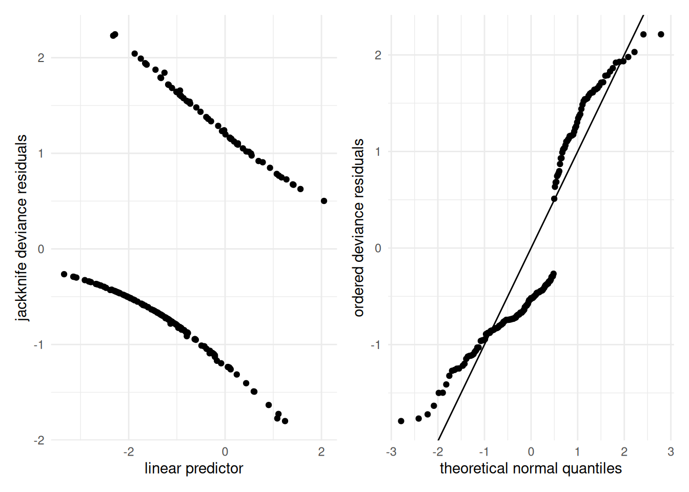
Figure B.1: Diagnostic plots for the binary regression for the birth weight data: jackknife deviance residuals against linear predictor (left) and quantile-quantile plot of ordered deviance residuals (right).

Another strategy is use of quantile residuals (Brillinger and Preisler 1983). If \(Y \sim F\), the quantile transform gives \(U=F(Y) \sim \mathsf{U}(0,1)\), meaning uniformly distributed on \((0,1)\). Replacing the unknown distribution \(F\) by \(\widehat{F}\) should yield approximately uniform observations. With \(\widehat{\pi}_i\) denoting the probability of success, we take \[\begin{align*} U_i = U_{i1} Y_i + U_{i2}(1-Y_i), \qquad U_{i1} \sim \mathsf{U}(0, \widehat{\pi}_i), \quad U_{i2} \sim \mathsf{U}(\widehat{\pi}_i, 1) \end{align*}\] and the resulting uniform residuals will be, as their name hints, approximately uniform on \((0,1)\). The drawback of this approach lies in the randomness of the residuals. Figure B.2 shows the diagnostic plots based on the uniform residuals (top two rows): there is no overall indication of poor fit, except for seemingly too few low/high residuals. The two observations with high leverage correspond to non-smoker mothers with no premature labour record: one with hypertension and a weight of 95lbs (unusual combination), the other weighting 200 lbs, with no hypertension and presence of uterine irritability.

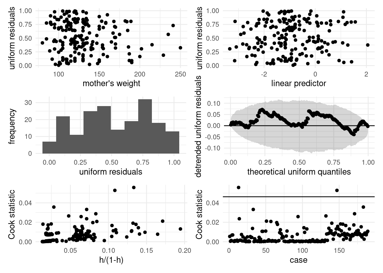
Figure B.2: Diagnostic plots based on uniform residuals for the birth weight data. From left to right, top to bottom: residuals against explanatory and linear predictors, histogram of uniform residuals and Tukey’s quantile-quantile plot, Cook statistic against weighted leverage and case number.

B.3 Restricted estimation maximum likelihood

The most common estimation technique for fitting linear mixed models or fixed effect models in which the variance of the error term is not \(\sigma^2\mathbf{I}_n\) is the restricted estimation maximum likelihood (REML) method.

For the linear mixed model, the marginal distribution of the \(n\) response vector is \(\boldsymbol{Y} \sim \mathsf{No}_n\{\mathbf{X} \boldsymbol{\beta}, \boldsymbol{\Upsilon}^{-1}(\boldsymbol{\psi})\}\), where \(\boldsymbol{\Upsilon}^{-1}(\boldsymbol{\psi}) = \mathbf{Z}\boldsymbol{\Omega}\mathbf{Z}^\top + \mathbf{R}\) and \(\mathbf{R} = \mathrm{blockdiag}(\mathbf{R}_1, \ldots, \mathbf{R}_m)\), the covariance matrix of the errors, is block-diagonal. The multivariate normal distribution has covariance parameters \(\boldsymbol{\psi}\) and mean parameters \(\boldsymbol{\beta}\).

The log likelihood for the model is, up to proportionality constants \[\begin{align*} \ell(\boldsymbol{\beta},\boldsymbol{\psi}; \boldsymbol{y}) \propto \frac{1}{2} \ln |\boldsymbol{\Upsilon}|- \frac{1}{2} (\boldsymbol{y}- \mathbf{X}\boldsymbol{\beta})^\top\boldsymbol{\Upsilon}(\boldsymbol{y}-\mathbf{X}\boldsymbol{\beta}) \end{align*}\]

For known \(\boldsymbol{\psi}\), the precision matrix \(\boldsymbol{\Upsilon}\) is fully resolved; the restricted maximum likelihood for the parameters of the mean vector \(\boldsymbol{\beta}\) is \[\begin{align*} \widehat{\boldsymbol{\beta}}_{\boldsymbol{\psi}} = (\mathbf{X}^\top\boldsymbol{\Upsilon}\mathbf{X})^{-1}\mathbf{X}^\top\boldsymbol{\Upsilon}\boldsymbol{y}. \end{align*}\] We can show that \(\widehat{\boldsymbol{\beta}}_{\boldsymbol{\psi}} \sim \mathsf{No}_{p+1}\{\boldsymbol{\beta}, (\mathbf{X}^\top\boldsymbol{\Upsilon}\mathbf{X})^{-1}\}\) and thus write the joint density of the response given mean and variance parameters as \[\begin{align*} f(\boldsymbol{y}; \boldsymbol{\psi}, \boldsymbol{\beta}) = f(\boldsymbol{y}; \widehat{\boldsymbol{\beta}}_{\boldsymbol{\psi}}, \boldsymbol{\beta}, \boldsymbol{\psi}) f(\widehat{\boldsymbol{\beta}}_{\boldsymbol{\psi}}; \boldsymbol{\psi}, \boldsymbol{\beta}). \end{align*}\] Given \(\boldsymbol{\psi}\), \(\widehat{\boldsymbol{\beta}}_{\boldsymbol{\psi}}\) is a sufficient statistic for \(\boldsymbol{\beta}\), the conditional density depends on \(\boldsymbol{\beta}\) only through \(\widehat{\boldsymbol{\beta}}_{\boldsymbol{\psi}}\), so \(f(\boldsymbol{y}; \widehat{\boldsymbol{\beta}}_{\boldsymbol{\psi}}, \boldsymbol{\beta}, \boldsymbol{\psi}) = f(\boldsymbol{y}; \widehat{\boldsymbol{\beta}}_{\boldsymbol{\psi}}, \boldsymbol{\psi})\). Rather than using the full likelihood, the REML maximizes the conditional log likelihood \[\begin{align*} \ell_{\mathrm{r}}(\boldsymbol{\psi})= \ln f(\boldsymbol{y}; \widehat{\boldsymbol{\beta}}_{\boldsymbol{\psi}}, \boldsymbol{\psi}) = \ln f(\boldsymbol{y}; \boldsymbol{\psi}, \boldsymbol{\beta}) - \ln f(\widehat{\boldsymbol{\beta}}_{\boldsymbol{\psi}}; \boldsymbol{\psi}, \boldsymbol{\beta}). \end{align*}\] The solution thus differs from that of the maximum log likelihood. The log conditional density is \[\begin{align*} \ell_{\mathrm{r}}(\boldsymbol{\psi}) &= \frac{1}{2} \ln |\boldsymbol{\Upsilon}| - \frac{1}{2} (\boldsymbol{y}-\mathbf{X}\boldsymbol{\beta})^\top\boldsymbol{\Upsilon}(\boldsymbol{y}-\mathbf{X}\boldsymbol{\beta}) \\& \quad - \frac{1}{2} \ln \left|\mathbf{X}^\top\boldsymbol{\Upsilon}\mathbf{X}\right| + \frac{1}{2} \left(\widehat{\boldsymbol{\beta}}_{\boldsymbol{\psi}}-\boldsymbol{\beta}\right)^\top \mathbf{X}^\top\boldsymbol{\Upsilon}\mathbf{X} \left(\widehat{\boldsymbol{\beta}}_{\boldsymbol{\psi}}-\boldsymbol{\beta}\right) \end{align*}\] and upon simplifying terms using the fact \(\boldsymbol{y} - \mathbf{X}\boldsymbol{\beta} = \boldsymbol{y} - \mathbf{X}\widehat{\boldsymbol{\beta}}_{\boldsymbol{\psi}} + \mathbf{X}(\widehat{\boldsymbol{\beta}}_{\boldsymbol{\psi}} - \boldsymbol{\beta})\), we retrieve the REML log likelihood, \[\begin{align*} \ell_{\mathrm{r}}(\boldsymbol{\psi}) = \frac{1}{2}|\boldsymbol{\Upsilon}| - \frac{1}{2} \ln \left|\mathbf{X}^\top\boldsymbol{\Upsilon}\mathbf{X}\right| - \frac{1}{2}(\boldsymbol{y} -\mathbf{X}\widehat{\boldsymbol{\beta}}_{\boldsymbol{\psi}})^\top \boldsymbol{\Upsilon}(\boldsymbol{y} -\mathbf{X}\widehat{\boldsymbol{\beta}}_{\boldsymbol{\psi}}) \end{align*}\] Once we have obtained \(\widehat{\boldsymbol{\psi}}_{\mathrm{r}}= \max_{\boldsymbol{\psi}} \ell_{\mathrm{r}}(\boldsymbol{\psi})\), we replace the resulting \(\widehat{\boldsymbol{\Upsilon}}\) value in \(\widehat{\boldsymbol{\beta}}_{\widehat{\boldsymbol{\psi}}_{\mathrm{r}}}\) to get the REML estimates. Because the estimation of \(\boldsymbol{\psi}\) is based on only part of the full likelihood, estimators for the covariance parameter differ from their counterpart based on the full likelihood; in practice, the latter are often more biased, which explains the popularity of REML. The sufficient statistic \(\widehat{\boldsymbol{\beta}}_{\widehat{\boldsymbol{\psi}}}\) depends on the particular model matrix \(\mathbf{X}\), so models with different fixed effects cannot be compared based on their maximum restricted likelihood values.

It should be noted that optimisation for linear mixed model is challenging for large \(n\) and direct matrix inversion must be avoided, as inverting a square \(n \times n\) matrix requires \(\mathrm{O}(n^3)\) flops. Software for mixed models must use clever tricks to capitalize on the sparsity of \(\boldsymbol{\Upsilon}\), which often follows from that of \(\mathbf{R}\); oftentimes \(\mathbf{R} = \sigma^2 \mathbf{I}_n\).