Solution 7
Exercise 7.1
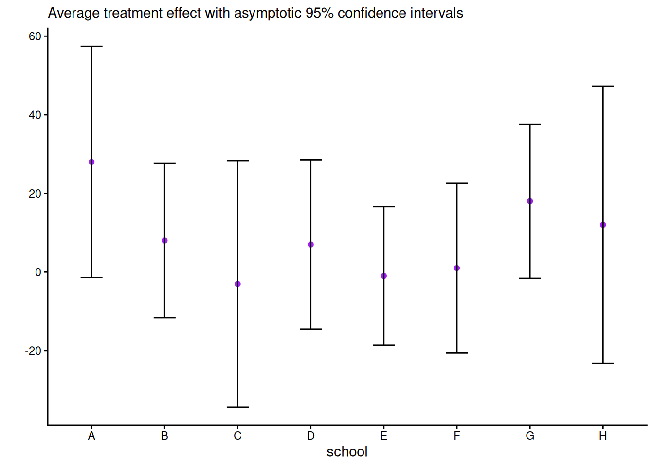
Consider the eight school data from Educational Testing Service (ETS), featured prominently in Gelman et al. (2013). The data shows results of randomized experiments in eight different schools to estimate the effect of coaching on SAT-V scores. The data consist of estimated treatment mean difference and their standard errors. The data size are large, so the average treatment effect (ATE) can be considered Gaussian and the standard errors are treated as a known quantity.
Derive the Gibbs sampler for the two models with improper priors. Note that, to sample jointly from \(p(\mu, \boldsymbol{\alpha} \mid \boldsymbol{y}, \sigma^2_{\alpha}, \boldsymbol{\sigma}^2_{\boldsymbol{y}})\), you can draw from the marginal of \(\boldsymbol{\alpha}\), then the conditional \(\mu \mid \boldsymbol{\alpha}, \cdots\).
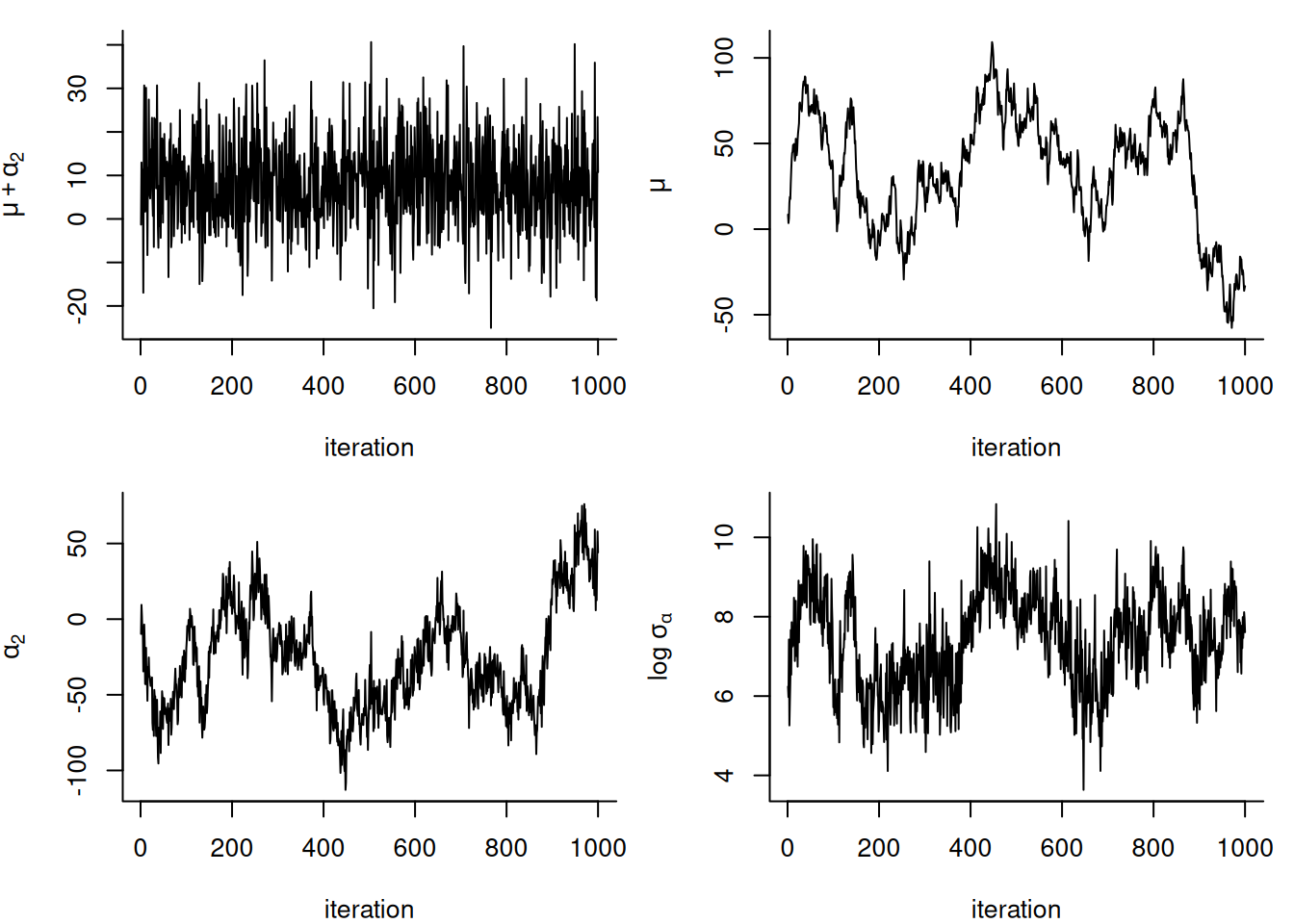
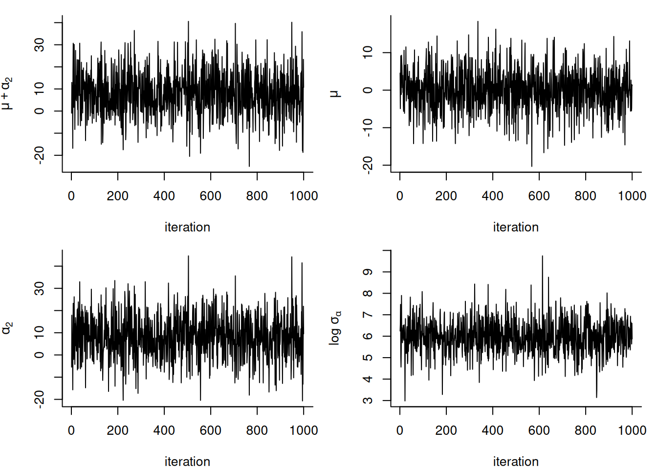
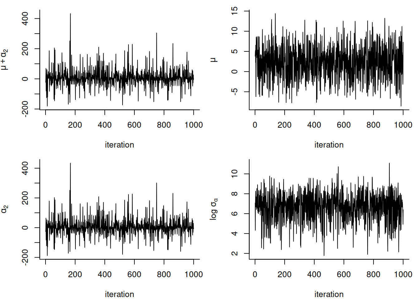
Fit the three algorithms described in Gelman et al. (2008) and compare their efficiency via effective sample size (ESS). In particular, draw traceplots and calculate effective sample sizes for
- \(\mu\)
- \(\alpha_1\),
- the sum \(\mu + \alpha_1\).
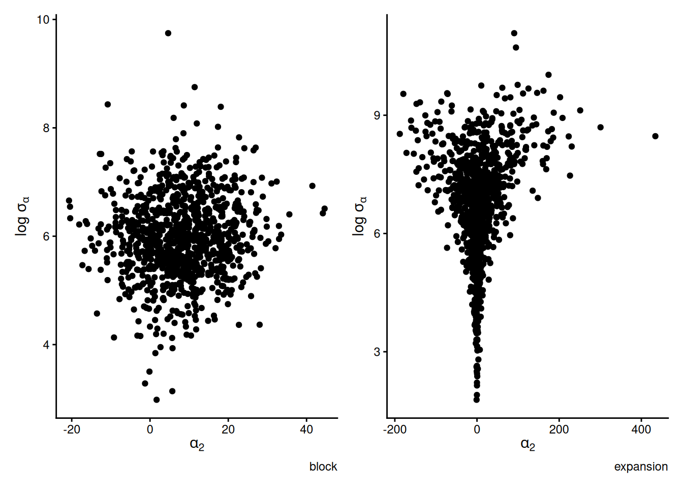
as well as pairs plot of \(\alpha_i, \log \sigma_{\alpha}\). The latter should display a very strong funnel.
Consider a one-way ANOVA with a single observation per group, where for \(i=1, \ldots, n,\) we have \[\begin{align*} Y_{i} &\sim \mathsf{Gauss}(\mu + \alpha_i, s^2_i) \\ \alpha_i &\sim \mathsf{Gauss}(0, \sigma^2_\alpha) \end{align*}\] and an improper prior for the mean \(p(\mu) \propto 1.\) If there are \(K\) groups, then the group-specific mean is \(\mu+\alpha_k\), and there is a redundant parameter. In the Bayesian setting, the parameters are weakly identifiable because of the prior on \(\boldsymbol{\alpha}\), but the geometry is such that \(\alpha_k \to 0\) as \(\sigma^2_{\alpha} \to 0.\) See Section 5.5 on p.119 of Gelman et al. (2013) for more details.
We fit the model by adding redundant parameter to improve mixing (Gelman et al., 2008) \[\begin{align*} Y_{i} &\sim \mathsf{Gauss}(\mu + \nu\xi_i, \sigma^2_i) \\ \xi_i &\sim \mathsf{Gauss}(0, \sigma^2_\xi) \end{align*}\] so that \(\alpha_i=\nu\xi_i\) and \(\sigma_\alpha = |\nu|\sigma_\xi.\)
See this post for display of the pathological behaviour that can be captured by divergence in Hamiltonian Monte Carlo.
Solution. If we use the matrix formulation and write \(\boldsymbol{S}^2 = \mathrm{diag}\{s_1^2, \ldots, s_n^2\}\) for the diagonal matrix of (fixed) sample variance, then the log of the joint density of \(p(\mu, \boldsymbol{\alpha} \mid \boldsymbol{y}, \boldsymbol{s}, \sigma_\alpha)\) is proportional to \[\begin{align*} \log p(\mu, \boldsymbol{\alpha} \mid \boldsymbol{y}, \boldsymbol{s}, \sigma_\alpha) &\propto -\frac{1}{2} (\boldsymbol{y} - \boldsymbol{\alpha} - \mathbf{1}_8\mu)^\top \boldsymbol{S}^{-2}(\boldsymbol{y} - \boldsymbol{\alpha} - \mathbf{1}_8\mu) - \frac{1}{2} \sum_{j=1}^8 \frac{\alpha_j^2}{\sigma_{\alpha}^2}\\ & \propto -\frac{1}{2}\left(\mu \mathbf{1}_8^{\top}\boldsymbol{S}^{-2}\mathbf{1}_8\mu + 2 (\boldsymbol{y} - \boldsymbol{\alpha})^\top \boldsymbol{S}^{-2}\mathbf{1}_8\mu + \sum_{j=1}^8 \frac{(y_i-\alpha_i)^2}{s_j^2} + \frac{\alpha_j^2}{\sigma_{\alpha}^2}\right). \end{align*}\] If we write \(s_\mu^{-2} = \sum_{j=1}^8 s_j^{-2} = \mathbf{1}_8^\top\boldsymbol{S}^{-2}\mathbf{1}_8\) for the precision of \(\mu \mid \cdot\), it is easy to complete the two quadratic forms to get \[\begin{align*} \mu \mid \boldsymbol{y}, \boldsymbol{s}^2, \boldsymbol{\alpha} & \sim \mathsf{Gauss}\left( s^2_{\mu} \sum_{j=1}^8 \frac{y_j-\alpha_j}{s^2_j}, s^2_{\mu}\right)\\ \alpha_i \mid y_i, s_i^2, \sigma^2_{\alpha} &\sim \mathsf{Gauss}\left\{\frac{y_is^{-2}_j}{s^{-2}_i + \sigma^{-2}_{\alpha}}, \left(s^{-2}_i + \sigma^{-2}_{\alpha}\right)^{-1}\right\} \end{align*}\]
If we use parameter expansion now and replace \(\alpha_i = \nu \xi_i\) and \(\sigma_{\alpha} = |\nu| \sigma_{\xi}\), the conditional are the same.
The other steps are detailed in Gelman et al. (2008).
# Eight school data
es <- data.frame(
  school = LETTERS[1:8],
  y = c(28, 8, -3, 7, -1, 1, 18, 12),
  se = c(15, 10, 16, 11, 9, 11, 10, 18)
)
n <- nrow(es)
B <- 1e3L
set.seed(80601)
# Starting values
alpha <- rnorm(0, sd = 0.01)
mu <- mean(es$y)
sigma_al <- sqrt(var(es$y) - mean(es$se))
pars1 <- matrix(NA, nrow = B, ncol = n + 2)
var_mu <- 1 / sum(1 / es$se^2)
# Sampler 1 - Gibbs with full conditionals
set.seed(80601)
for (b in seq_len(B)) {
  var_al <- 1 / (1 / es$se^2 + 1 / sigma_al^2)
  pars1[b, 1:n] <- alpha <- rnorm(
    n = n,
    mean = var_al * (es$y - mu) / es$se^2,
    sd = sqrt(var_al)
  )
  pars1[b, n + 1] <- mu <- rnorm(
    n = 1,
    mean = var_mu * sum((es$y - alpha) / es$se^2),
    sd = sqrt(var_mu)
  )
  pars1[b, n + 2] <- sigma_al <- sum(alpha^2) / rchisq(1, df = n - 1)
}

## Sampler 2
# Same model, with joint updates
set.seed(80601)
# Starting values
alpha <- rnorm(0, sd = 0.01)
mu <- mean(es$y)
sigma_al <- sqrt(var(es$y) - mean(es$se))
pars2 <- matrix(NA, nrow = B, ncol = n + 2)
for (b in seq_len(B)) {
  var_al <- 1 / (1 / es$se^2 + 1 / sigma_al^2)
  # Sample from joint of alpha, mu
  # by taking p(alpha | sigma_al, y) *
  # p(mu | alpha, sigma_al, y)
  pars2[b, 1:n] <- alpha <- rnorm(
    n = n,
    mean = var_al * es$y / es$se^2,
    sd = sqrt(var_al)
  )
  pars2[b, n + 1] <- mu <- rnorm(
    n = 1,
    mean = var_mu * sum((es$y - alpha) / es$se^2),
    sd = sqrt(var_mu)
  )
  pars2[b, n + 2] <- sigma_al <-
    sum(alpha^2) / rchisq(1, df = n - 1)
}

# Parameter expansion - V+PX sampler
a <- 1
pars3 <- matrix(NA, nrow = B, ncol = n + 3)
for (b in seq_len(B)) {
  var_al <- 1 / (1 / es$se^2 + 1 / sigma_al^2)
  # Sample from joint of alpha, mu
  # by taking p(alpha | sigma_al, y) * p(mu | alpha, sigma_al, y)
  alpha_st <- rnorm(
    n = n,
    mean = var_al * es$y / es$se^2,
    sd = sqrt(var_al)
  )
  pars3[b, n + 1] <- mu <- rnorm(
    n = 1,
    mean = var_mu * sum((es$y - alpha) / es$se^2),
    sd = sqrt(var_mu)
  )
  pars3[b, n + 2] <- sigma_al_st <-
    sum(alpha_st^2) / rchisq(1, df = n - 1)
  pars3[b, n + 3] <- a <- rnorm(
    n = 1,
    mean = sum(alpha_st * (es$y - mu) / es$se^2) /
      sum(alpha_st^2 / es$se^2),
    sd = sqrt(sum(alpha_st^2 / es$se^2))
  )
  pars3[b, 1:n] <- alpha_st * a
  pars3[b, n + 2] <- sigma_al <- abs(a) * sigma_al_st
}
References
Gelman, A., Carlin, J. B., Stern, H. S., Dunson, D. B., Vehtari, A., & Rubin, D. B. (2013). Bayesian data analysis (3rd ed.). Chapman; Hall/CRC. https://doi.org/10.1201/b16018
Gelman, A., Dyk, D. A. van, Huang, Z., & Boscardin, J. W. (2008). Using redundant parameterizations to fit hierarchical models. Journal of Computational and Graphical Statistics, 17(1), 95–122. https://doi.org/10.1198/106186008x287337