data(SKD23_S2A, package = "hecedsm") # load data
linmod <- lm(pef ~ proportion, data = SKD23_S2A)
# fit simple linear regression
coef(linmod) # extract intercept and slope
(Intercept) proportion
2.4073939 0.5264168 If factors measure a continuous quantity, we may alternatively consider a statistical model that describes a curve or a straight line, rather than only determining the mean at the levels measured in an experiment. These types of experiments are rather common in engineering.
Example 9.1 (Is additional paper wrapping viewed as more eco-friendly?) Sokolova, Krishna, and Döring (2023) consider consumer bias when assessing how eco-friendly packages are. Items such as cereal are packaged in plastic bags, which themselves are covered in a box. They conjecture (and find) that, paradoxically, consumers tend to view the packaging as being more eco-friendly when the amount of cardboard or paper surrounding the box is larger, relative to the sole plastic package. We consider in the sequel the data from Study 2A, which measures the perceived environmental friendliness (PEF, variable pef) as a function of the proportion of paper wrapping (either none, half of the area of the plastic, equal or twice).
The linear model we can envision measures the effect of pef as a linear function of proportion, with \[\begin{align*}
\mathsf{E}(\texttt{pef} \mid \texttt{proportion}) = \beta_0 + \beta_1 \texttt{proportion}
\end{align*}\] and with homoscedastic observations. More general models would include polynomials (up to degree \(K-1\) for a factor with \(K\) levels).
If we fit against the simple linear regression model, we can extract the estimated coefficients and the \(p\)-values for the \(t\)-test for \(\beta_0\) and \(\beta_1\). The test for the intercept is of no interest since data are measured on a scale from 1 to 7, so the mean response when proportion=0 cannot be zero. The coefficient for proportion suggests a trend of 0.5 point per unit ratio, and this is significantly different from zero, indicating that the pef score changes with the paper to plastic ratio.
data(SKD23_S2A, package = "hecedsm") # load data
linmod <- lm(pef ~ proportion, data = SKD23_S2A)
# fit simple linear regression
coef(linmod) # extract intercept and slope(Intercept) proportion
2.4073939 0.5264168 Let \(\mu_{0}, \mu_{0.5}, \mu_{1}, \mu_2\) denote the true mean of the PEF score as a function of the proportion of paper. There are several tests that could be of interest here, but we focus on contrasts performed by authors and an hypothesis test of linearity as a function of the proportion of plastic. For the latter, we could compare the linear regression model (in which the PEF score increases linearly with the proportion of paper to plastic) against the ANOVA which allows each of the four groups to have different means.
If we use \(\boldsymbol{\alpha} \in \mathbb{R}^4\) to denote the parameter vector of the analysis of variance model using the treatment parametrization and \(\boldsymbol{\beta} \in \mathbb{R}^2\) for the simple linear regression model, then we have \[\begin{align*} \mu_0 &= \beta_0=\alpha_0 \\ \mu_{0.5} &= \beta_0 + 0.5 \beta_1 = \alpha_0 + \alpha_1\\ \mu_1 &= \beta_0 + \beta_1 = \alpha_0 + \alpha_2 \\ \mu_2 &= \beta_0 + 2 \beta_1= \alpha_0 + \alpha_3. \end{align*}\] The test comparing the simple linear regression with the analysis of variance imposes two simultaneous restrictions, with \(\mathscr{H}_0: \alpha_3 = 2\alpha_2= 4\alpha_1\), so the null distribution is \(\mathsf{Fisher}(2, 798)\) or roughly \(\chi^2_2\).
anovamod <- lm(pef ~ factor(proportion), # one-way ANOVA
               data = SKD23_S2A)
# Compare simple linear regression with ANOVA
anova(linmod, anovamod) # is the change in PEF linear?
Analysis of Variance Table
Model 1: pef ~ proportion
Model 2: pef ~ factor(proportion)
Res.Df RSS Df Sum of Sq F Pr(>F)
1 800 1372.7
2 798 1343.4 2 29.262 8.6909 0.0001845 ***
---
Signif. codes: 0 '***' 0.001 '**' 0.01 '*' 0.05 '.' 0.1 ' ' 1# Specifying the weights
# these contrasts encode the mean (so don't sum to zero)
car::linearHypothesis(model = anovamod,
hypothesis = rbind(c(0, -2, 1, 0),
c(0, 0, -2, 1)))
Linear hypothesis test:
- 2 factor(proportion)0.5  + factor(proportion)1 = 0
- 2 factor(proportion)1  + factor(proportion)2 = 0

Model 1: restricted model
Model 2: pef ~ factor(proportion)

  Res.Df    RSS Df Sum of Sq      F    Pr(>F)
1    800 1372.7
2    798 1343.4  2    29.262 8.6909 0.0001845 ***
---
Signif. codes:  0 '***' 0.001 '**' 0.01 '*' 0.05 '.' 0.1 ' ' 1
We see from the output that the \(F\) tests and the \(p\)-values are identical, whether we impose the constraints manually or simply feed the two nested models to the anova method.
The authors were interested in comparing none with other choices: we are interested in pairwise differences, but only relative to the reference \(\mu_{0}\): \[\begin{align*} \mu_0 = \mu_{0.5} & \iff 1\mu_0 - 1\mu_{0.5} + 0\mu_{1} + 0 \mu_{2} = 0\\ \mu_0 = \mu_{1} & \iff 1\mu_0 + 0\mu_{0.5} -1\mu_{1} + 0 \mu_{2} = 0\\ \mu_0 = \mu_{2} & \iff 1\mu_0 + 0\mu_{0.5} + 0\mu_{1} -1 \mu_{2} = 0 \end{align*}\] so contrast vectors \((1, -1, 0, 0)\), \((1, 0, -1, 0)\) and \((1, 0, 0, -1)\) for the marginal means would allow one to test the hypothesis.
margmean <- anovamod |>
  emmeans::emmeans(specs = "proportion") # group means
contrastlist <- list( # specify contrast vectors
   refvshalf = c(1, -1, 0, 0),
   refvsone =  c(1, 0, -1, 0),
   refvstwo =  c(1, 0, 0, -1))
# compute contrasts relative to reference
margmean |> emmeans::contrast(method = contrastlist)
contrast estimate SE df t.ratio p.value
refvshalf -0.749 0.131 798 -5.713 <.0001
refvsone -0.901 0.131 798 -6.893 <.0001
refvstwo -1.182 0.129 798 -9.196 <.0001The group averages are reported in Table 9.1, match those reported by the authors in the paper. They suggest an increased perceived environmental friendliness as the amount of paper used in the wrapping increases. We could fit a simple regression model to assess the average change, treating the proportion as a continuous explanatory variable. The estimated slope for the change in PEF score, which ranges from 1 to 7 in increments of 0.25, is 0.53 point per ratio of paper/plastic. There is however strong evidence, given the data, that the change isn’t quite linear, as the fit of the linear regression model is significantly worse than the corresponding linear model.
| proportion | marg. mean | std. err. | dof | lower (CI) | upper (CI) |
|---|---|---|---|---|---|
| 0.0 | 2.16 | 0.093 | 798 | 1.98 | 2.3439 |
| 0.5 | 2.91 | 0.093 | 798 | 2.73 | 3.0926 |
| 1.0 | 3.06 | 0.092 | 798 | 2.88 | 3.2441 |
| 2.0 | 3.34 | 0.089 | 798 | 3.17 | 3.5193 |
| contrast | estimate | std. err. | dof | stat | p-value |
|---|---|---|---|---|---|
| refvshalf | -0.75 | 0.13 | 798 | -5.71 | 0 |
| refvsone | -0.90 | 0.13 | 798 | -6.89 | 0 |
| refvstwo | -1.18 | 0.13 | 798 | -9.20 | 0 |
All differences reported in Table 9.2 are significant and positive, in line with the researcher’s hypothesis.
The previous chapter dealt with factorial experiments in which all experimental factors are of interest. It is possible to use measurements concomitant to the data collection (for example, value to a test before we complete the group assignment for the manipulation) to get a measure of the relative strength of students. The more correlated these measures are with the response, the more we can explain the data. We then proceed with the random assignment of our experimental units to different conditions.
Including covariates should in principle increase power and our ability to detect real differences due to experimental manipulations, provided the variables used as control are correlated with the response. Generally, they are not needed for valid inference, which is guaranteed by randomization, and shouldn’t be used to assign treatment. Such designs are meant to reduce the error.
We can include continuous covariates to the analysis of variance, whose slope governs the relationship with the response. The strict inclusion isn’t necessary to draw valid causal conclusion, but adding the term helps again reduce the residual variability. Such a design was historically called analysis of covariance, although as analysis of variance models, they are nothing but linear regression models. The ANCOVA model assumes that slopes are parallel: if rather there is an interaction term, then the experimental manipulation induces changes that depend on the value of the continuous explanatory. This case is termed moderation in the management literature.
In an analysis of covariance, we include a linear component for a (continuous) covariate, with the purpose again to reduce residual error and increase power. A prime example is prior/post experiment measurements, whereby we monitor the change in outcome due to the manipulation. This post by Solomon Kurz [link] nicely illustrates the added benefits of using covariates when there is strong correlation between your response and the latter
In such setting, it may seem logical to take the difference in post and prior score as response: this is showcased in Example 9.3 and Baumann, Seifert-Kessell, and Jones (1992), an analysis of which is presented on the course website.
When we add a covariate, we need the latter to have a strong linear correlation for the inclusion to make sense. We can assess graphically whether the relationship is linear, and whether the slopes for each experimental condition are the same.1
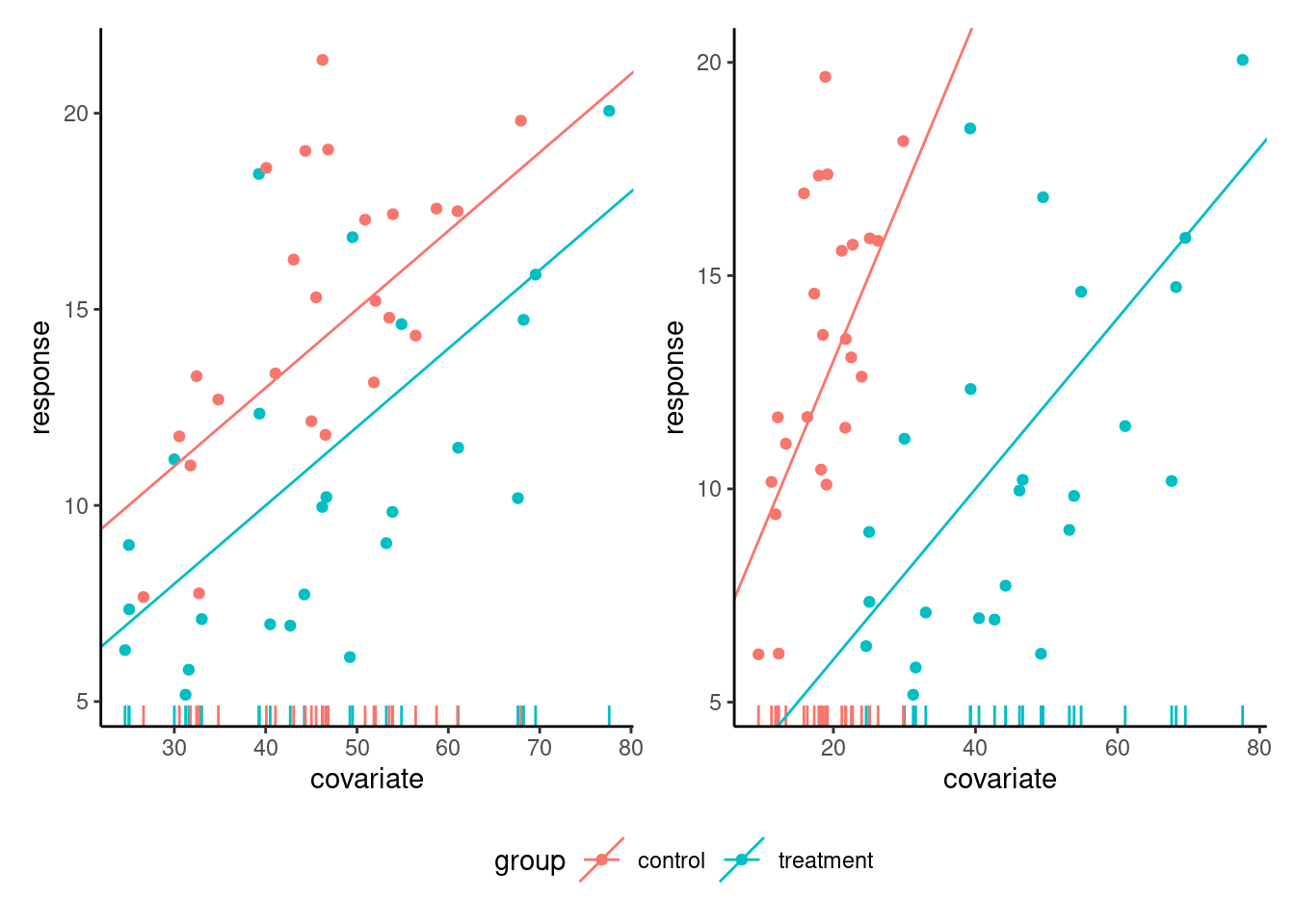
The left panel of Figure 9.1 shows the ideal situation for an analysis of covariate: the relationship between response and covariate is linear with strong correlation, with the same slope and overlapping support. Since the slopes are the same, we can compare the difference in average (the vertical difference between slopes at any level of the covariate) because the latter is constant, so this depiction is useful. By contrast, the right-hand panel of Figure 9.1 shows an interaction between the covariate and the experimental groups, different slopes: there, the effect of the experimental condition increases with the level of the covariate. One may also note that the lack of overlap in the support, the set of values taken by the covariate, for the two experimental conditions, makes comparison hazardous at best in the right-hand panel.
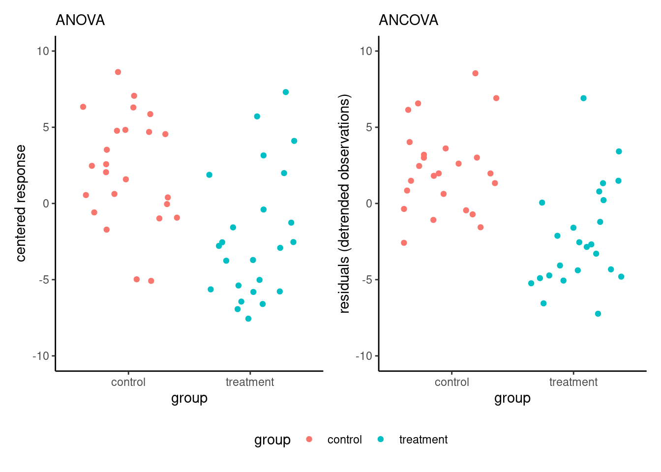
Figure 9.2 shows that, due to the strong correlation, the variability of the measurements is smaller on the right-hand panel (corresponding to the analysis of covariance model) than for the centred response on the left-hand panel; note that the \(y\)-axes have different scales.
We present two examples of analysis of covariance, showing how the inclusion of covariates helps disentangle differences between experimental conditions.
Example 9.2 (Inconsistency of product description and image in online retailing) Lee and Choi (2019) measured the impact of discrepancies between descriptions and visual depiction of items in online retail. They performed an experiment in which participants were presented with descriptions of a product (a set of six toothbrushes) that was either consistent or inconsistent with the description. The authors postulated that a discrepancy could lead to lower appreciation score, measured using three Likert scales. They also suspected that the familiarity with the product brand should impact ratings, and controlled for the latter using another question.
One way to account for familiarity when comparing the mean is to use a linear regression with familiarity as another explanatory variable. The expected value of the product evaluation is \[ \mathsf{E}(\texttt{prodeval}) = \beta_0 + \beta_1 \texttt{familiarity} + \beta_2 \texttt{consistency}, \tag{9.1}\] where \(\texttt{familiarity}\) is the score from 1 to 7 and \(\texttt{consistency}\) is a binary indicator equal to one if the output is inconsistent and zero otherwise. The coefficient \(\beta_2\) thus measures the difference between product evaluation rating for consistent vs inconsistent displays, for the same familiarity score.
We can look at coefficient (standard error) estimates \(\widehat{\beta}_2 = -0.64 (0.302)\). No difference between groups would mean \(\beta_2=0\) and we can build a test statistic by looking at the standardized regression coefficient \(t = \widehat{\beta}_2/\mathsf{se}(\widehat{\beta}_2)\). The result output is \(b = -0.64\), 95% CI \([-1.24, -0.04]\), \(t(93) = -2.12\), \(p = .037\). We reject the null hypothesis of equal product evaluation for both display at level 5%: there is evidence that there is a small difference, with people giving on average a score that is 0.64 points smaller (on a scale of 1 to 9) when presented with conflicting descriptions and images.
We can compare the analysis of variance table obtained by fitting the model with and without \(\texttt{familiarity}\). Table 9.3 shows that the effect of consistency is small and not significant and a two-sample t-test shows no evidence of difference between the average familiarity score in both experimental conditions (\(p\)-value of \(.532\)). However, we can explain roughly one fifth of the residual variability by the familiarity with the brand (see the sum of squares in Table 9.3): removing the latter leads to a higher signal-to-noise ratio for the impact of consistency, at the expense of a loss of one degree of freedom. Thus, it appears that the manipulation was successful.
| term | sum. sq. | df | stat | p-value |
|---|---|---|---|---|
| consistency | 7.04 | 1 | 2.55 | .113 |
| Residuals | 259.18 | 94 |
| term | sum. sq. | df | stat | p-value |
|---|---|---|---|---|
| familiarity | 55.94 | 1 | 25.60 | < .001 |
| consistency | 9.80 | 1 | 4.49 | .037 |
| Residuals | 203.24 | 93 |
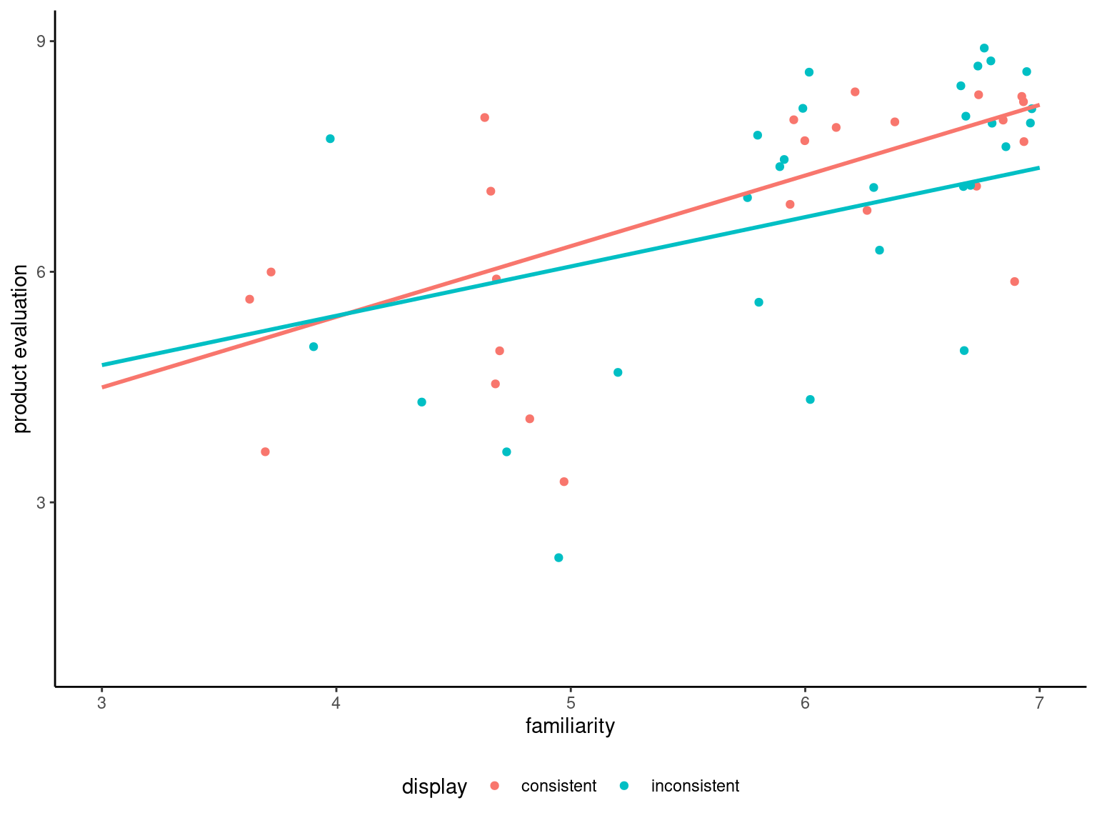
Figure 9.3 shows that people more familiar with the product or brand tend to have a more positive product evaluation, as postulated by the authors. The graph also shows two straight lines corresponding to the fit of a linear model with different intercept and slope for each display group: there is little material difference, one needs to assess formally whether a single linear relationship as the one postulated in Equation 9.1 can adequately characterize the relation in both groups.
To this effect, we fit a linear model with different slopes in each group, and compare the fit of the latter with the analysis of covariance model that includes a single slope for both groups: we can then test if the slopes are the same, or alternatively if the difference between the slopes is zero. The t-statistic indicates no difference in slope (\(p\)-value of \(.379\)), thus the assumption is reasonable. Levene’s test for homogeneity of variance indicates no discernible difference between groups. Thus, it appears there is a difference in perception of product quality due to the manipulation.
Example 9.3 (Effect of scientific consensus on false beliefs) We consider Study 3 of Stekelenburg et al. (2021), who studied changes in perception of people holding false beliefs or denying (to some extent) the scientific consensus by presenting them with news article showcasing information about various phenomena. The experimental manipulation consisted in presenting boosting, a form of training to help readers identify and establish whether scientifists were truly expert in the domain of interest, how strong was the consensus, etc.2
The third and final experiment of the paper focused on genetically modified organisms: it is a replication of Study 2, but with a control group (since there were no detectable difference between experimental conditions Boost and BoostPlus) and a larger sample size (because Study 2 was underpowered).
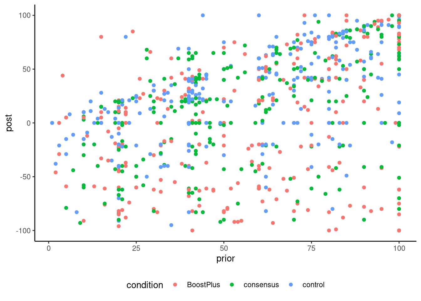
The data include 854 observations with prior, the negative of the prior belief score of the participant, the post experiment score for the veracity of the claim. Both were measured using a visual scale ranging from -100 (I am 100% certain this is false) to 100 (I am 100% certain this is true), with 0 (I don’t know) in the middle. Only people with negative prior beliefs were recruited to the study. The three experimental conditions were BoostPlus, consensus and a control group. Note that the scores in the data have been negated, meaning that negative posterior scores indicate agreement with the consensus on GMO.
Preliminary checks suggest that, although the slopes for prior beliefs could plausibly be the same in each group and the data are properly randomized, there is evidence of unequal variance for the changes in score. As such, we fit a model with mean \[\begin{align*} \mathsf{E}(\texttt{post}) &= \begin{cases} \beta_0 + \beta_1 \texttt{prior} + \alpha_1 & \texttt{condition} = \texttt{BoostPlus}\\ \beta_0 + \beta_1 \texttt{prior} + \alpha_2 &\texttt{condition} = \texttt{consensus}\\ \beta_0 + \beta_1 \texttt{prior} + \alpha_3 &\texttt{condition} = \texttt{control} \end{cases} \end{align*}\] with \(\alpha_1 + \alpha_2 + \alpha_3=0\), using the sum-to-zero parametrization, and with different variance for each experimental condition, \[\begin{align*} \mathsf{Va}(\texttt{post}) = \begin{cases} \sigma^2_1, & \texttt{condition} = \texttt{BoostPlus},\\ \sigma^2_2, & \texttt{condition} = \texttt{consensus},\\ \sigma^2_3, & \texttt{condition} = \texttt{control}. \end{cases} \end{align*}\] Because of the unequal variances, we cannot use multiple testing procedures reserved for analysis of variance and resort instead to Holm–Bonferroni to control the familywise error rate. We here look only at pairwise differences between conditions.3
| term | df | stat | p-value |
|---|---|---|---|
| condition | 2 | 42.5 | < .001 |
| term | df | stat | p-value |
|---|---|---|---|
| prior | 1 | 289.2 | < .001 |
| condition | 2 | 57.0 | < .001 |
Repeating the exercise of comparing the amount of evidence for comparison with and without inclusion of a covariate shows that the value of the test statistic is larger (Table 9.4), indicative of stronger evidence with the analysis of covariance model: the conclusion would be unaffected with such large sample sizes. We of course care very little for the global \(F\) test of equality of mean, as the previous study had shown large differences. What is more interesting here is quantifying the change between conditions.
| contrast | estimate | std.error | df | statistic | p.value |
|---|---|---|---|---|---|
| consensus vs control | -11.98 | 4.0 | 557.54 | -3.007 | .003 |
| consensus vs BoostPlus | 16.31 | 4.7 | 546.36 | 3.490 | < .001 |
| BoostPlus vs control | -28.29 | 4.4 | 505.44 | -6.489 | < .001 |
| contrast | estimate | std.error | df | statistic | p.value |
|---|---|---|---|---|---|
| consensus vs control | -11.84 | 3.3 | 543.06 | -3.544 | < .001 |
| consensus vs BoostPlus | 17.47 | 4.3 | 523.60 | 4.108 | < .001 |
| BoostPlus vs control | -29.30 | 3.9 | 458.62 | -7.454 | < .001 |
Table 9.5 shows the pairwise contrasts, which measure two different things: the analysis of variance model compares the average in group, whereas the analysis of covariance (the linear model with prior) uses detrended values and focuses on the change in perception. Because the data are unbalanced and we estimate group mean and variance separately, the degrees of freedom change from one pairwise comparison to the next. Again, using the covariate prior, which is somewhat strongly correlated with post as seen in Figure 9.4, helps decrease background noise.
| time | condition | mean | se |
|---|---|---|---|
| prior | BoostPlus | 57.65 | 1.69 |
| prior | consensus | 56.32 | 1.67 |
| prior | control | 56.49 | 1.68 |
| post | BoostPlus | 2.62 | 3.53 |
| post | consensus | 18.93 | 3.06 |
| post | control | 30.91 | 2.56 |
Stekelenburg et al. (2021) split their data to do pairwise comparisons two at the time (thus taking roughly two-third of the data to perform a two sample t-test with each pair). Although it does not impact their conclusion, this approach is conceptually incorrect: if the variance was equal, we would want to use all observations to estimate it (so their approach would be suboptimal, since we would estimate the variance three times with smaller samples).
On the contrary, using a model that assumes equal variance when it is not the case leads to distortion: the variance we estimate will be some sort of average of the variability \(\sigma_i\) and \(\sigma_j\) in experimental condition \(i\) and \(j\), again potentially leading to distortions. With large samples, this may be unconsequential, but illustrates caveats of subsample analyses.
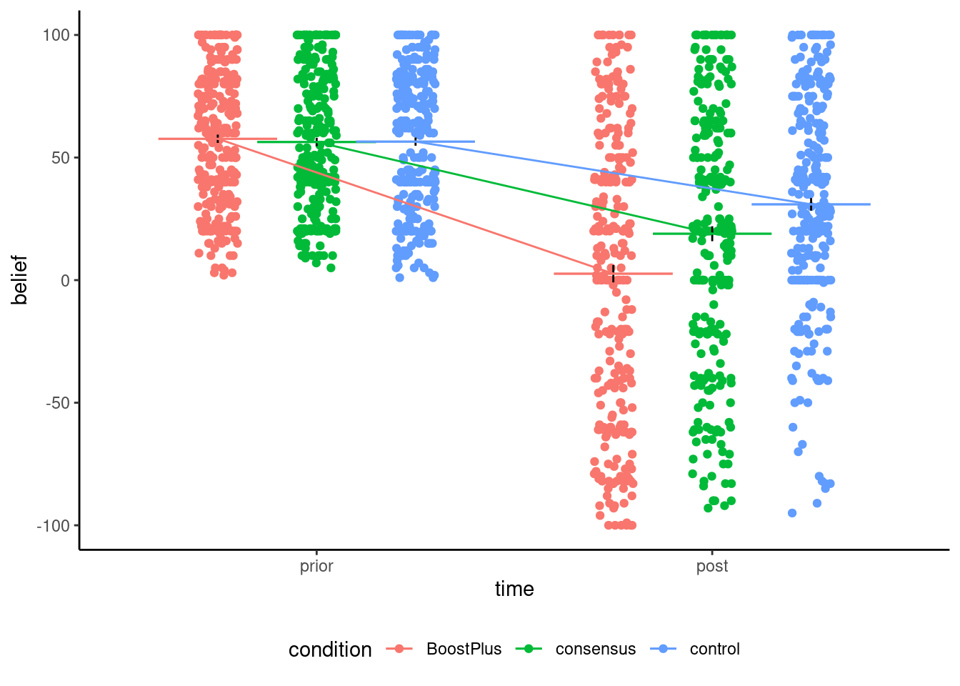
Figure 9.5 shows the relationship between prior and posterior score. The data show clear difference between individuals: many start from completely disbelieving of genetically engineered food and change their mind (sometimes drastically), there are many people who do not change idea at all and have similar scores, and many who give a posterior score of zero. This heterogeneity in the data illustrates the danger of only looking at the summary statistics and comparing averages. It does not tell the whole picture! One could investigate whether the strength of religious or political beliefs, or how much participants trust scientists, could explain some of the observed differences.
In a randomized experiment, we can check the average outcome of a manipulation by comparing groups: assuming random sampling, these conclusions can be broadly generalized to the population of interest from which the sample is drawn. However, it may be that the effect of the treatment depends on other variables: cultural differences, gender or education may change.
The causal effect on \(Y\) of the experimental manipulation, say \(X\) may be a misleading summary if another variable modifies the relation of \(X \to Y\): for example, the perception of gender discrimination or racism may depend on the person background and experience and this may impact the effect of the manipulation. Such variables, say \(W\), thus have an interactive effect with the experimental factor \(X\), termed moderator in psychology. In the statistical model, inclusion of interaction terms between \(X\) and \(W\) (typically via product of the so-called moderator variable with the factor encoding the experimental sub-condition) will allow us to estimate those differences.
In an analysis of covariance, covariates are included that have an impact on the outcome to filter out variability, but with the assumption that they do not influence the effect of treatment (no interaction). With moderators, we rather include and tests for the interactions. If we have an experimental factor \(X\) which is binary or categorical, the resulting model is a simple analysis of variance model (or analysis of covariance) and we can test the significance of the interaction term to assess the moderating effect of \(W\).
If \(W\) is a mean-centered continuous variable and \(X\) a categorical variable with \(k=1, \ldots, K\) levels using the sum-to-zero parametrization, the linear model with mean \[ \underset{\text{average response at $W$ in group $k$}}{\mathsf{E}\{Y \mid \mathsf{do}(X) = k, W\}} = \underset{\text{intercept for group $k$}}{\mu + \alpha_k} + \underset{\text{slope for group $k$}}{(\beta + \gamma_k)}W \] includes different slopes for \(W\) in each experimental group, as well as different intercepts for each group.
Example 9.4 (Gender discrimation) We consider data from a study on gender discrimination (Garcia et al. 2010). Participants were put with a file where a women was turned down promotion in favour of male colleague despite her being clearly more experimented and qualified. The authors manipulated the decision of the participant to this decision, either choosing not to challenge the decision (no protest), a request to reconsider based on individual qualities of the applicants (individual) and a request to reconsider based on abilities of women (collective). All items were measured using scales constructed using items measured using Likert scales ranging from strongly disagree (1) to strongly agree (7).
The postulated mediator variable is sexism, the average of 6 Likert scales for the Modern Sexism Scale assessing pervasiveness of gender discrimination. We consider participants’ evaluation of the appropriateness of the response of the fictional character.
We fit the linear model with the interaction and display the observed slopes
data(GSBE10, package = "hecedsm")
lin_moder <- lm(respeval ~ protest*sexism,
               data = GSBE10)
summary(lin_moder) # coefficients
car::Anova(lin_moder, type = 3) # tests| term | sum of squares | df | stat | p-value |
|---|---|---|---|---|
| protest | 6.34 | 2 | 2.45 | .091 |
| sexism | 6.59 | 1 | 5.09 | .026 |
| protest:sexism | 12.49 | 2 | 4.82 | .010 |
| Residuals | 159.22 | 123 |
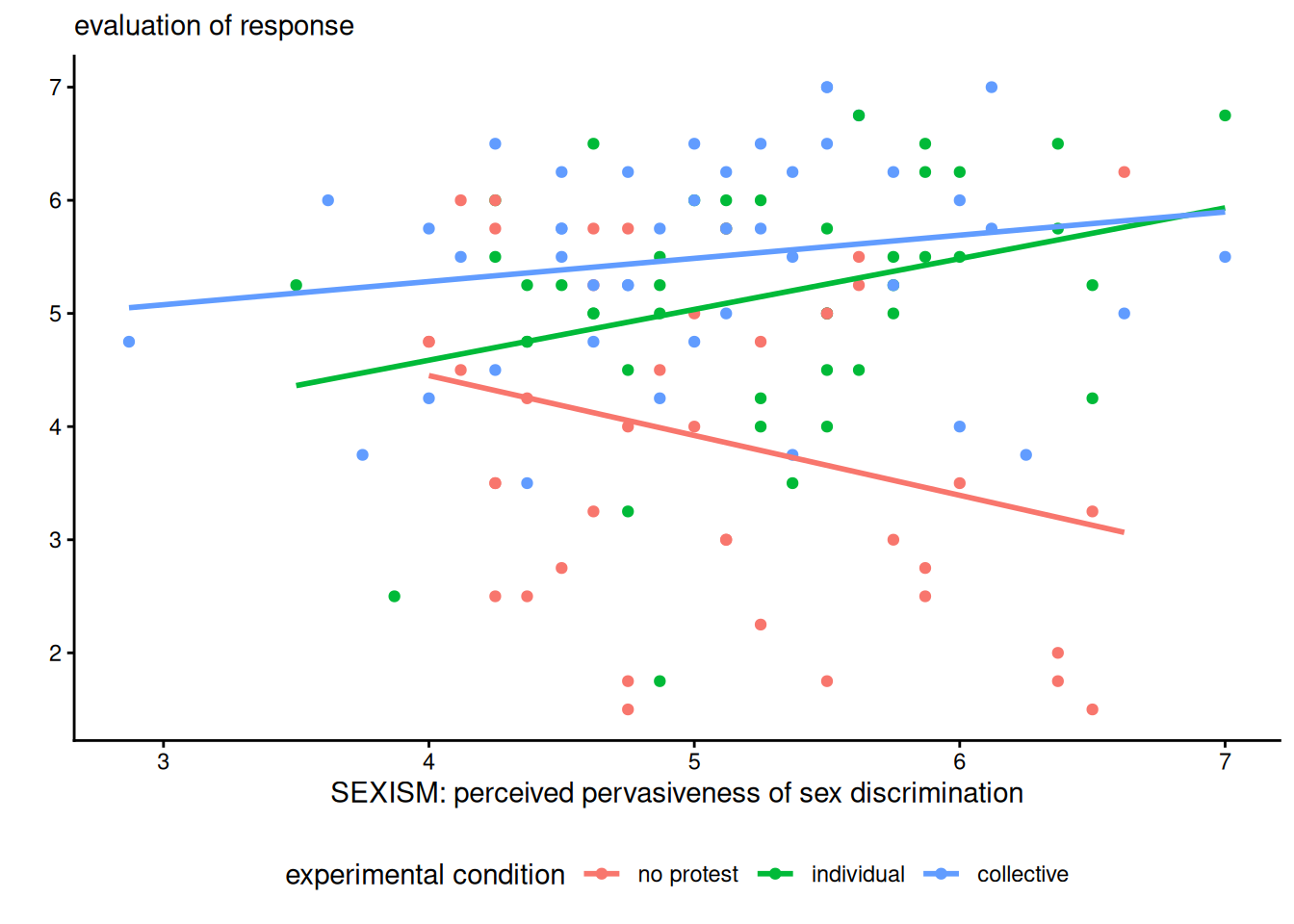
Because of the interaction, comparing the levels of the experimental factor only makes sense if we fix the value of sexism (since the slopes are not parallel) and won’t necessarily be reliable outside of the range of observed values of sexism. We could look at quantiles and differences at the mean sexism,4 or one standard deviation away.
We may be interested in the range of values of the predictor \(W\) for which the difference between treatments is not statistically significant if we only have a binary treatment. The Johnson–Neyman method (Johnson and Neyman 1936) considers this range, but this leads to multiple testing problems since we probe the model repeatedly. Esarey and Sumner (2018) offer a method that provides control for the false discovery rate.
To illustrate the method, we dichotomize the manipulation pooling individual and collective protests, since these are the most similar.
library(interactions)
db <- GSBE10 |>
  dplyr::mutate(
    protest = as.integer(protest != "no protest"))
lin_moder2 <- lm(respeval ~ protest*sexism, data = db)
jn <- johnson_neyman(
  model = lin_moder2, # linear model
  pred = protest, # binary experimental factor
  modx = sexism, # moderator
  control.fdr = TRUE,
  mod.range = range(db$sexism))
jn$plot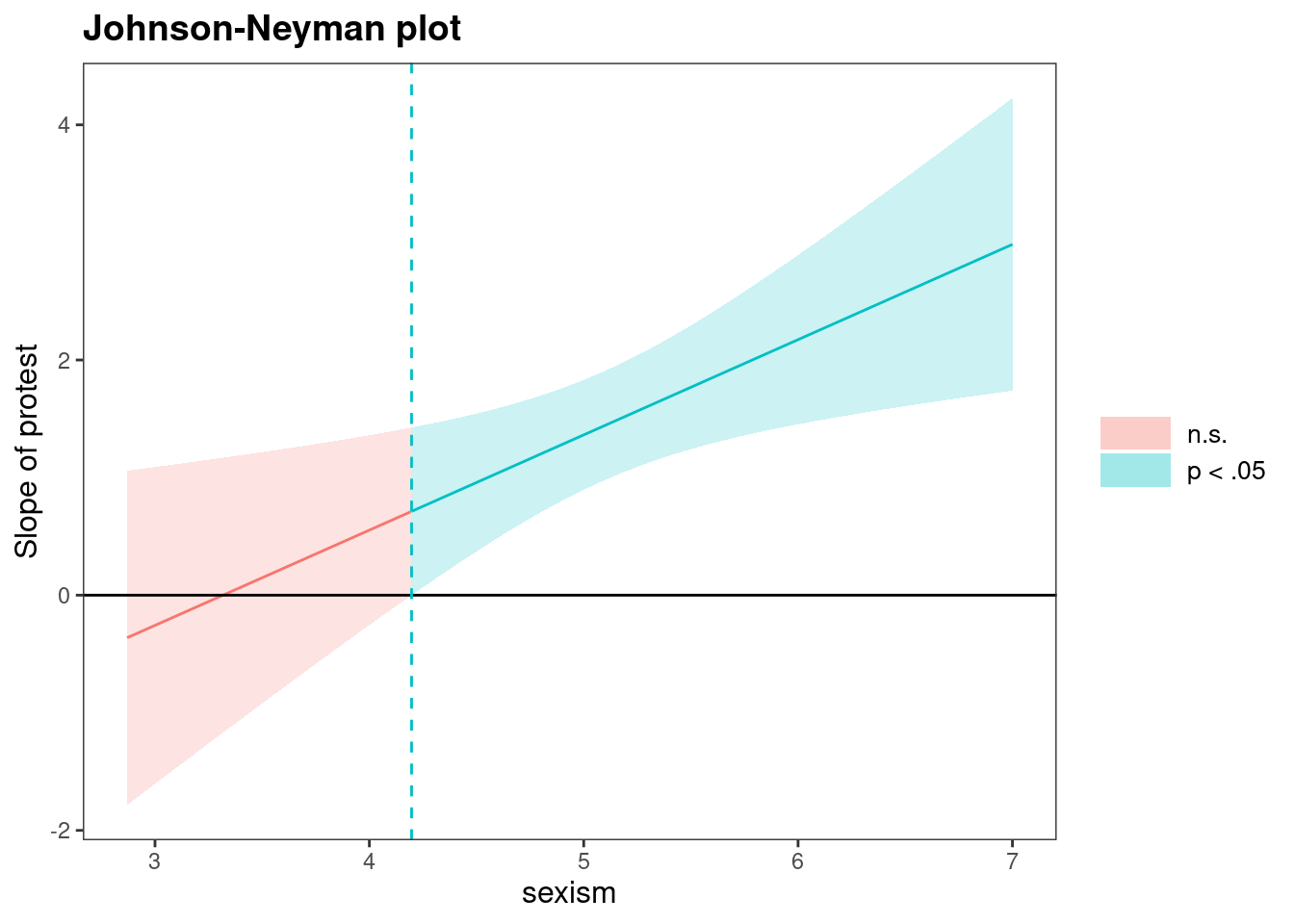
The cutoff value is 4.20 with control for the false discovery rate and 4.15 without. The interval is not extended beyond the range of value for sexism, as these are not possible given the Likert scale (which starts at 1). In this example, the moderator is not experimentally manipulated, but it could be. More complicated mediation models could include interactions between treatment effects or moderators and covariates, with external variables, leading to moderated mediation. Interactions can be considered for pretty much any statistical model, but the usual assumptions need to hold for inference to be approximately valid.
Example 9.5 (Ghosting) Leckfor et al. (2023) consider the impact of ghosting someone (i.e., not responding to communications and cutting bridges with a person) on personal satisfaction, uncertainty and the need for closure (explanations). In their Study 3, they postulated that the type of rejection someone experienced. The study comprises 545 participants who were asked to reflect about a situation in their own life, in scenarios where
Participants in the included (control) condition were asked to write about a time when someone “expressed that they wanted to continue and/or maintain a friendship, romantic relationship, or casual dating situation.” Participants in the ghosted condition wrote about a time when someone ended a relationship by “suddenly cutting off all communication without explanation.” Participants in the directly rejected condition wrote about a time when someone “directly communicate[d] that they wanted to end the relationship.” Nearly half (49%) of participants wrote about a friendship, followed by a romantic relationship (29%), and then a casual dating situation (22%).
The moderator variable is cond, one of control, being ghosted or rejected. This should moderate the effect of the need for closure on need for satisfaction. The authors postulated that individuals would have lower needs of satisfaction after being ghosted.
# Moderation analysis
# This time, the factor of interest is continuous
# and the moderator is categorical (K=3 levels)
data(LWSH23_S3, package = "hecedsm")
mod <- lm(data = LWSH23_S3, needsatis ~ needclosure * cond)
anova(mod) # interaction is significant
# Compute estimated marginal means, but with global weights equal to relative weight of each variable
emmeans::emmeans(mod, specs = "needclosure",
                 by = "cond",
                 at = list(needclosure = 2:7),
                 weights = "prop")
# All values are reported for the average of needclosure by default without the at| term | coef. | estimate | std. error | lower CL | upper CL |
|---|---|---|---|---|---|
| (Intercept) | \(\beta_0\) | 5.0 | 0.37 | 4.29 | 5.74 |
| need for closure | \(\beta_1\) | 0.2 | 0.07 | 0.04 | 0.33 |
| directly rejected [cond] | \(\beta_2\) | -1.2 | 0.53 | -2.20 | -0.12 |
| ghosted [cond] | \(\beta_3\) | -1.5 | 0.50 | -2.48 | -0.52 |
| need for closure * directly rejected [cond] | \(\beta_4\) | -0.4 | 0.11 | -0.61 | -0.19 |
| need for closure * ghosted [cond] | \(\beta_5\) | -0.4 | 0.10 | -0.62 | -0.21 |
| term | df | sum of squares | stat | p-value |
|---|---|---|---|---|
| needclosure | 1 | 3.9 | 4.26 | .039 |
| cond | 2 | 1346.9 | 738.61 | < .001 |
| needclosure:cond | 2 | 18.6 | 10.19 | < .001 |
| Residuals | 539 | 491.5 |
Since the interaction is significant, we focus on the different slopes. We can of course simply report the equations of the linear regression for each group. Alternative, emmeans can also return the predictions for different values of needclosure per condition along with standard errors. The estimates will have lower values of needclosure when close to the subgroup averages.
The postulated theoretical mean equation is \[\begin{align*}
\mathsf{E}(\texttt{needsatisf}) &= \beta_0 + \beta_1\texttt{needclosure} + \beta_2 \mathsf{1}_{\texttt{cond=directly rejected}} +\beta_3 \mathsf{1}_{\texttt{cond=directly rejected}} \\&+ \beta_4 \texttt{needclosure} \times \mathsf{1}_{\texttt{cond=directly rejected}} +\beta_5 \texttt{needclosure} \times\mathsf{1}_{\texttt{cond=directly rejected}}.
\end{align*}\] The estimated model mean \(\widehat{\mathsf{E}}(\texttt{needsatisf} \mid \texttt{needclosure}=x)\) when needclosure is worth \(x \in [1,7]\) for each cond is thus \[\begin{align*}
\widehat{Y} & = \begin{cases}
\widehat{\beta}_0 + \widehat{\beta}_1x, & \texttt{control};\\
(\widehat{\beta}_0 + \widehat{\beta}_3) + (\widehat{\beta}_1 + \beta_4)x , & \texttt{directly rejected};\\
(\widehat{\beta}_0 + \widehat{\beta}_2) + (\widehat{\beta}_1 + \beta_5)x, & \texttt{ghosted}.
\end{cases} \\&= \begin{cases}
5.015 + 0.181 x, & \texttt{control};\\
3.86 -0.222x, & \texttt{directly rejected};\\
3.52 -0.234x, & \texttt{ghosted}.
\end{cases}
\end{align*}\]
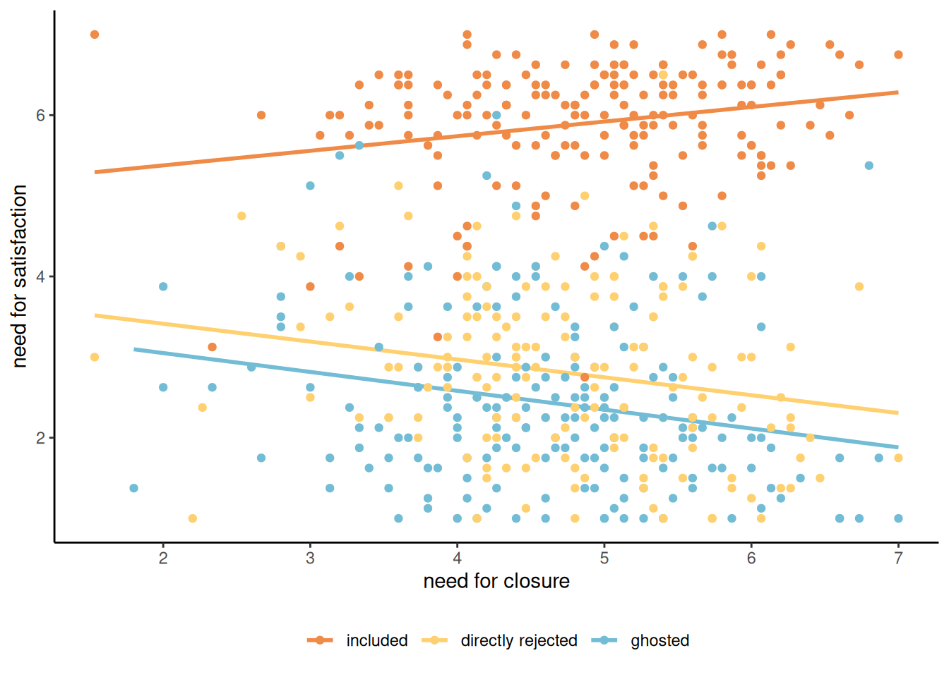
We can see clearly in Figure 9.7 that the impact of the need for closure depends on the situation, with downward trends for the ghosted and rejected groups.
We can fit this toy model also with the PROCESS macro, which only understand numeric values for factors… The output (omitted) includes model coefficients with confidence intervals, the \(F\) test statistic for the ANOVA, and output for the average need for closure.
process(data = LWSH23_S3 |>
          dplyr::mutate(condind = as.integer(cond)), # cast factor to numeric integer levels
        y = "needsatis",  # response variable
        x = "needclosure", # explanatory variable (not manipulated)
        w = "condind", # postulated moderator
        mcw = 1, # dummy coding for moderator w (so compare to base level, here 'included')
model = 1) # number of model in Hayes (simple moderation)If not, this implies that the covariate interacts with the experimental condition.↩︎
The article is interesting because lack of planning/changes led them to adapt the design from experiment 1 to 3 until they found something. Without preregistration, it is unlikely such findings would have been publishable.↩︎
In Study 2, the interest was comparing manipulation vs control and the Boost vs BoostPlus conditions, two orthogonal contrasts.↩︎
This is the default with emmeans↩︎