4  Contrasts and multiple testing

Key concept

Learning objectives:

• Specifying contrast weights to test for differences between groups
• Understanding the problem of multiple testing and the danger for selective reporting
• Adjusting for multiple testing to control the global error rate.

4.1 Contrasts

Suppose we perform an analysis of variance and the \(F\)-test for the (global) null hypothesis that the averages of all groups are equal is very large: we reject the null hypothesis in favor of the alternative, which states that at least one of the group average is different. The follow-up question will be where these differences lie. Indeed, in an experimental context, this implies one or more of the manipulation has a different effect from the others on the mean response. Oftentimes, this isn’t interesting in itself: we could be interested in comparing different options relative to a status quo (e.g., for new drugs or medical treatment), or determine whether specific combinations work better than separately, or find the best treatment by comparing all pairs.

The scientific question of interest that warranted the experiment may lead to a specific set of hypotheses, which can be formulated by researchers as comparisons between means of different subgroups. We can normally express these as contrasts. As Dr. Lukas Meier puts it, if the global \(F\)-test for equality of means is equivalent to a dimly lit room, contrasts are akin to spotlight that let one focus on particular aspects of differences in treatments.

Formally speaking, a contrast is a linear combination of averages: in plain English, this means we assign a weight to each group average and add them up, and then compare that summary to a postulated value \(a\), typically zero. Contrasts encode research question of interest: if \(c_i\) denotes the weight of group average \(\mu_i\) \((i=1, \ldots, K)\), then we can write the contrast as \(C = c_1 \mu_1 + \cdots + c_K \mu_K\) with the null hypothesis \(\mathscr{H}_0: C=a\) for a two-sided alternative. The sample estimate of the linear contrast is obtained by replacing the unknown population average \(\mu_i\) by the sample average of that group, \(\widehat{\mu}_i = \overline{y}_{i}\). We can easily obtain the standard error of the linear combination \(C.\)¹ We can then build a \(t\) statistic as usual by looking at the difference between our postulated value and the observed weighted mean, suitably standardized. If the global \(F\)-test leads to rejection of the null, there exists a contrast which is significant at the same level.

4.1.1 Orthogonal contrasts

Sometimes, linear contrasts encode disjoint bits of information about the sample: for example, one contrast that compares groups the first two groups versus one that compares the third and fourth is in effect using data from two disjoint samples, as contrasts are based on sample averages. Whenever the contrasts vectors are orthogonal, the tests will be uncorrelated. Mathematically, if we let \(c_{i}\) and \(c^{*}_{i}\) denote weights attached to the mean of group \(i\) comprising \(n_i\) observations, contrasts are orthogonal if \(c_{1}c^{*}_{1}/n_1 + \cdots + c_{K}c^{*}_K/n_K = 0\); if the sample is balanced with the same number of observations in each group, \(n/K = n_1 =\cdots = n_K\), we can consider the dot product of the two contrast vectors and neglect the subsample sizes.

If we have \(K\) groups, there are \(K-1\) contrasts for pairwise differences, the last one being captured by the sample mean for the overall effect². If we care only about difference between groups (as opposed to the overall effect of all treatments), we impose a sum-to-zero constraint on the weights so \(c_1 + \cdots + c_K=0\). Keep in mind that, although independent tests are nice mathematically, contrasts should encode the hypothesis of interest to the researchers: we choose contrasts because they are meaningful, not because they are orthogonal.

Example 4.1 (Contrasts for encouragement on teaching) The arithmetic data example considered five different treatment groups with 9 individuals in each. Two of them were control groups, one received praise, another was reproved and the last was ignored.

Suppose that researchers were interested in assessing whether the experimental manipulation had an effect, and whether the impact of positive and negative feedback is the same on students.³

Suppose we have five groups in the order (control 1, control 2, praised, reproved, ignored). We can express these hypothesis as

• \(\mathscr{H}_{01}\): \(\mu_{\text{praise}} = \mu_{\text{reproved}}\)
• \(\mathscr{H}_{02}\): \[\begin{align*} \frac{1}{2}(\mu_{\text{control}_1}+\mu_{\text{control}_2}) = \frac{1}{3}\mu_{\text{praised}} + \frac{1}{3}\mu_{\text{reproved}} + \frac{1}{3}\mu_{\text{ignored}} \end{align*}\]

Note that, for the hypothesis of control vs experimental manipulation, we look at average of the different groups associated with each item. Using the ordering, the weights of the contrast vector are \((1/2, 1/2, -1/3, -1/3, -1/3)\) and \((0, 0, 1, -1, 0)\). There are many equivalent formulation: we could multiply the weights by any number (different from zero) and we would get the same test statistic, as the latter is standardized.

library(emmeans)
data(arithmetic, package = "hecedsm")
linmod <- aov(score ~ group, data = arithmetic)
linmod_emm <- emmeans(linmod, specs = 'group')
contrast_specif <- list(
  controlvsmanip = c(0.5, 0.5, -1/3, -1/3, -1/3),
  praisedvsreproved = c(0, 0, 1, -1, 0)
)
contrasts_res <- 
  contrast(object = linmod_emm, 
                    method = contrast_specif)
# Obtain confidence intervals instead of p-values
confint(contrasts_res)

Table 4.1: Contrasts estimates for the arithmetic data

contrast	estimate	std. error	df	lower (CI)	upper (conf. limit)CI)
control vs manip	-3.33	1.05	40	-5.45	-1.22
praised vs reproved	4.00	1.62	40	0.72	7.28

Example 4.2 (Teaching to read) We consider data from Baumann, Seifert-Kessell, and Jones (1992). The abstract of the paper provides a brief description of the study

This study investigated the effectiveness of explicit instruction in think aloud as a means to promote elementary students’ comprehension monitoring abilities. Sixty-six fourth-grade students were randomly assigned to one of three experimental groups: (a) a Think-Aloud (TA) group, in which students were taught various comprehension monitoring strategies for reading stories (e.g., self-questioning, prediction, retelling, rereading) through the medium of thinking aloud; (b) a Directed reading-Thinking Activity (DRTA) group, in which students were taught a predict-verify strategy for reading and responding to stories; or (c) a Directed reading Activity (DRA) group, an instructed control, in which students engaged in a noninteractive, guided reading of stories.

Looking at Table 4.2, we can see that DRTA has the highest average, followed by TA and directed reading (DR).

library(emmeans) #load package
data(BSJ92, package = "hecedsm")
mod_post <- aov(posttest1 ~ group, data = BSJ92)
emmeans_post <- emmeans(object = mod_post, 
                        specs = "group")

Table 4.2: Estimated group averages with standard errors and 95% confidence intervals for post-test 1.

terms	marg. mean	std. err.	dof	lower (CI)	upper (CI)
DR	6.68	0.68	63	5.32	8.04
DRTA	9.77	0.68	63	8.41	11.13
TA	7.77	0.68	63	6.41	9.13

The purpose of Baumann, Seifert-Kessell, and Jones (1992) was to make a particular comparison between treatment groups. From the abstract:

The primary quantitative analyses involved two planned orthogonal contrasts—effect of instruction (TA + DRTA vs. 2 x DRA) and intensity of instruction (TA vs. DRTA)—for three whole-sample dependent measures: (a) an error detection test, (b) a comprehension monitoring questionnaire, and (c) a modified cloze test.

The hypothesis of Baumann, Seifert-Kessell, and Jones (1992) is \(\mathscr{H}_0: \mu_{\mathrm{TA}} + \mu_{\mathrm{DRTA}} = 2 \mu_{\mathrm{DRA}}\) or, rewritten slightly, \[\begin{align*} \mathscr{H}_0: - 2 \mu_{\mathrm{DR}} + \mu_{\mathrm{DRTA}} + \mu_{\mathrm{TA}} = 0. \end{align*}\] with weights \((-2, 1, 1)\); the order of the levels for the treatment are (\(\mathrm{DRA}\), \(\mathrm{DRTA}\), \(\mathrm{TA}\)) and it must match that of the coefficients. An equivalent formulation is \((2, -1, -1)\) or \((1, -1/2, -1/2)\): in either case, the estimated differences will be different (up to a constant multiple or a sign change). The vector of weights for \(\mathscr{H}_0: \mu_{\mathrm{TA}} = \mu_{\mathrm{DRTA}}\) is (\(0\), \(-1\), \(1\)): the zero appears because the first component, \(\mathrm{DRA}\) doesn’t appear. The two contrasts are orthogonal since \((-2 \times 0) + (1 \times -1) + (1 \times 1) = 0\).

# Identify the order of the level of the variables
with(BSJ92, levels(group))

[1] "DR"   "DRTA" "TA"  

# DR, DRTA, TA (alphabetical)
contrasts_list <- list(
  "C1: DRTA+TA vs 2DR" = c(-2, 1, 1), 
  # Contrasts: linear combination of means, coefficients sum to zero
  # 2xDR = DRTA + TA => -2*DR + 1*DRTA + 1*TA = 0 and -2+1+1 = 0
  "C1: average (DRTA+TA) vs DR" = c(-1, 0.5, 0.5), 
  #same thing, but halved so in terms of average
  "C2: DRTA vs TA" = c(0, 1, -1),
  "C2: TA vs DRTA" = c(0, -1, 1) 
  # same, but sign flipped
)
contrasts_post <- 
  contrast(object = emmeans_post,
           method = contrasts_list)
contrasts_summary_post <- summary(contrasts_post)

Table 4.3: Estimated contrasts for post-test 1.

contrast	estimate	std. err.	dof	stat	p-value
C1: DRTA+TA vs 2DR	4.18	1.67	63	2.51	0.01
C1: average (DRTA+TA) vs DR	2.09	0.83	63	2.51	0.01
C2: DRTA vs TA	2.00	0.96	63	2.08	0.04
C2: TA vs DRTA	-2.00	0.96	63	-2.08	0.04

We can look at these differences; since DRTA versus TA is a pairwise difference, we could have obtained the \(t\)-statistic directly from the pairwise contrasts using pairs(emmeans_post). Note that the two different ways of writing the comparison between DR and the average of the other two methods yield different point estimates, but same inference (i.e., the same \(p\)-values). For contrast \(C_{1b}\), we get half the estimate (but the standard error is also halved) and likewise for the second contrasts we get an estimate of \(\mu_{\mathrm{DRTA}} - \mu_{\mathrm{TA}}\) in the first case (\(C_2\)) and \(\mu_{\mathrm{TA}} - \mu_{\mathrm{DRTA}}\): the difference in group averages is the same up to sign.

What is the conclusion of our analysis of contrasts? It looks like the methods involving teaching aloud have a strong impact on reading comprehension relative to only directed reading. The evidence is not as strong when we compare the method that combines directed reading-thinking activity and thinking aloud.

Example 4.3 (Paper or plastic) Sokolova, Krishna, and Döring (2023) consider consumer bias when assessing how eco-friendly packages are. Items such as cereal are packaged in plastic bags, which themselves are covered in a box. They conjecture (and find) that consumers tend to view the packaging as being more eco-friendly when the amount of cardboard or paper surrounding the box is large, relative to the sole plastic package. We consider the data Study 2A, which measures the perceived environmental friendliness (PEF) as a function of the proportion of paper wrapping (either none, half of the area of the plastic, equal or twice). The authors are interested in comparing none with other choices.

If \(\mu_{0}, \mu_{0.5}, \mu_{1}, \mu_2\) denote the true mean of the PEF score as a function of the proportion of paper, we are interested in pairwise differences, but only relative to the reference \(\mu_{0}\): \[\begin{align*} \mu_0 = \mu_{0.5} & \iff 1\mu_0 - 1\mu_{0.5} + 0\mu_{1} + 0 \mu_{2} = 0\\ \mu_0 = \mu_{1} & \iff 1\mu_0 + 0\mu_{0.5} -1\mu_{1} + 0 \mu_{2} = 0\\ \mu_0 = \mu_{2} & \iff 1\mu_0 + 0\mu_{0.5} + 0\mu_{1} -1 \mu_{2} = 0 \end{align*}\] so contrast vectors \((1, -1, 0, 0)\), \((1, 0, -1, 0)\) and \((1, 0, 0, -1)\) would allow one to test the hypothesis.

data(SKD23_S2A, package = "hecedsm") # load data
linmod <- lm(pef ~ proportion, data = SKD23_S2A) # fit simple linear regression
anova(linmod) # check for significance of slope
coef(linmod) # extract intercept and slope
anovamod <- lm(pef ~ factor(proportion), data = SKD23_S2A) # one-way ANOVA
margmean <- anovamod |>  emmeans::emmeans(specs = "proportion") # group means
contrastlist <- list( # specify contrast vectors
   refvshalf = c(1, -1, 0, 0),
   refvsone =  c(1, 0, -1, 0),
   refvstwo =  c(1, 0, 0, -1))
# compute contrasts relative to reference 
margmean |> emmeans::contrast(method = contrastlist)

The group averages are reported in Table 4.4, match those reported by the authors in the paper. They suggest an increased perceived environmental friendliness as the amount of paper used in the wrapping increases. We could fit a simple regression model to assess the average change, treating the proportion as a continuous explanatory variable. The estimated slope for the change in PEF score, which ranges from 1 to 7 in increments of 0.25, is 0.53 per area of paper. There is however strong evidence, given the data, that the change isn’t quite linear, as the fit of the linear regression model is significantly worse than the corresponding linear model.

Table 4.4: Estimated group averages of PEF per proportion with standard errors

proportion	marg. mean	std. err.	dof	lower (CI)	upper (CI)
0.0	2.16	0.093	798	1.98	2.34
0.5	2.91	0.093	798	2.73	3.09
1.0	3.06	0.092	798	2.88	3.24
2.0	3.34	0.089	798	3.17	3.52

Table 4.5: Estimated contrasts for differences of PEF to no paper.

contrast	estimate	std. err.	dof	stat	p-value
refvshalf	-0.75	0.13	798	-5.71	0
refvsone	-0.90	0.13	798	-6.89	0
refvstwo	-1.18	0.13	798	-9.20	0

All differences reported in Table 4.5 are significant and positive, in line with the researcher’s hypothesis.

4.2 Multiple testing

Beyond looking at the global null, we will be interested in a set of contrast statistics and typically this number can be large-ish. There is however a catch in starting to test multiple hypothesis at once.

If you do a single hypothesis test and the testing procedure is well calibrated (meaning that the model model assumptions hold), \(p\)-values are generated uniformly on the interval \([0,1]\) and there is a probability of \(\alpha\) of making a type I error (i.e., concluding in favour of the alternative and rejecting the null incorrectly) if the null is true. The problem of the above approach is that the more tests you perform, the higher the chance of finding (incorrectly) something: with 20 independent tests, we expect that, on average, one of them will yield a \(p\)-value less than 5% even if this is a fluke. The problem with multiple testing is not so much that it occurs, but more than researchers tend to report selectively findings and only give the results of tests for which \(p \leq \alpha\), even if these are typically the product of chance. This makes most findings will not replicate: if we rerun the experiment, we will typically not find the same result.

There is an infinite potential number of contrasts with more than two factos. Not all tests are of interest: standard software will report all possible pairwise comparisons, but this may not be of interest as showcased in Example 4.4. If there are \(K\) groups to compare and any comparison is of interest, than we could performs \(\binom{K}{2}\) pairwise comparisons with \(\mathscr{H}_{0}: \mu_i = \mu_j\) for \(i \neq j\). For \(K=3\), there are three such comparisons, 10 pairwise comparisons if \(K=5\) and 45 pairwise comparisons if \(K=10\). The number of pairwise comparisons grows quickly.

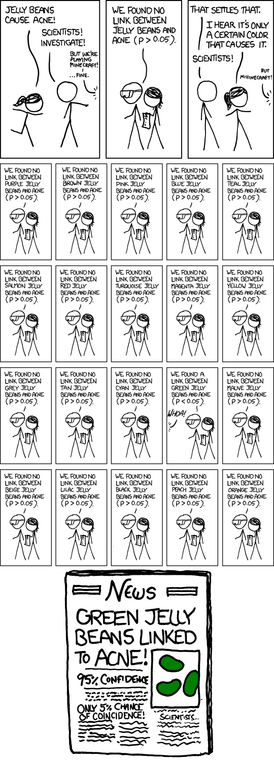
The number of tests performed in the course of an analysis can be very large. Y. Benjamini investigated the number of tests performed in each study of the Psychology replication project (Nosek et al. 2015): this number ranged from 4 to 700, with an average of 72 — most studies did not account for the fact they were performing multiple tests or selected the model and thus some ‘discoveries’ are bound to be spurious. It is natural to ask then how many results are spurious findings that correspond to type I errors. The paramount (absurd) illustration is the cartoon presented in Figure 4.1: note how there is little scientific backing for the theory (thus such test shouldn’t be of interest to begin with) and likewise the selective reporting made of the conclusions, despite nuanced conclusions.

We can also assess mathematically the problem. Assume for simplicity that all tests are independent⁴, then the probability of any rejecting the null incorrectly is \(\alpha\), but larger over the collection (with tests \(A\) and \(B\), we could reject by mistake if \(A\) is a type I error and \(B\) isn’t, or vice-versa, or if both are incorrect rejections.

The probability of making at least one type I error if each test is conducted at level \(\alpha\), say \(\alpha^{\star}\), is⁵ \[\begin{align} \alpha^{\star} &= 1 - \text{probability of making no type I error} \\ &= 1- (1-\alpha)^m \\ & \leq m\alpha \end{align}\]

With \(\alpha = 5\)% and \(m=4\) tests, \(\alpha^{\star} \approx 0.185\) whereas for \(m=72\) tests, \(\alpha^{\star} \approx 0.975\): this means we are almost guaranteed even when nothing is going on to find “statistically significant” yet meaningless results.

Figure 4.1: xkcd 882: Significant. The alt text is ‘So, uh, we did the green study again and got no link. It was probably a–’ ‘RESEARCH CONFLICTED ON GREEN JELLY BEAN/ACNE LINK; MORE STUDY RECOMMENDED!’

It is sensible to try and reduce or bound the number of false positive or control the probability of getting spurious findings. We consider a family of \(m\) null hypothesis \(\mathscr{H}_{01}, \ldots, \mathscr{H}_{0m}\), i.e. a collection of \(m\) hypothesis tests. The exact set depends on the context, but this comprises all hypothesis that are scientifically relevant and could be reported. These comparisons are called pre-planned comparisons: they should be chosen before the experiment takes place and pre-registered to avoid data dredging and selective reporting. The number of planned comparisons should be kept small relative to the number of parameters: for a one-way ANOVA, a general rule of thumb is to make no more comparisons than the number of groups, \(K\).

Suppose that we perform \(m\) hypothesis tests in a study and define binary indicators \[\begin{align} R_i &= \begin{cases} 1 & \text{if we reject the null hypothesis } \mathscr{H}_{0i} \\ 0 & \text{if we fail to reject } \mathscr{H}_{0i} \end{cases}\\ V_i &=\begin{cases} 1 & \text{type I error for } \mathscr{H}_{0i}\quad (R_i=1 \text{ and }\mathscr{H}_{0i} \text{ is true}) \\ 0 & \text{otherwise}. \end{cases} \end{align}\] With this notation, \(R=R_1 + \cdots + R_m\) simply encodes the total number of rejections (\(0 \leq R \leq m\)), and \(V = V_1 + \cdots + V_m\) is the number of null hypothesis rejected by mistake (\(0 \leq V \leq R\)).

The familywise error rate is the probability of making at least one type I error for the whole collection or test, in other words per family, is \[\begin{align*} \mathsf{FWER} = \Pr(V \geq 1). \end{align*}\] To control the familywise error rate, one must be more stringent in rejecting the null and perform each test with a smaller level \(\alpha\) so that the overall or simultaneous probability is less than \(\mathsf{FWER}\).

4.2.1 Bonferroni’s procedure

The easiest way to control for multiple testing is to perform each test at level \(\alpha/m\), thereby ensuring that the family-wise error is controlled at level \(\alpha\). This is a good option if \(m\) is small and the Bonferroni adjustment also controls the per-family error rate, which is the expected (theoretical average) number of false positive \(\mathsf{PFER} = \mathsf{E}(V)\). The latter is a more stringent criterion than the familywise error rate because \(\Pr(V \geq 1) \leq \mathsf{E}(V)\): the familywise error rate does not make a distinction between having one or multiple type I errors.⁶

Why is Bonferroni’s procedure popular? It is conceptually easy to understand and simple, and it applies to any design and regardless of the dependence between the tests. However, the number of tests to adjust for, \(m\), must be prespecified and the procedure leads to low power when the size of the family is large, meaning it makes detection of non-null effects more difficult. Moreover, if our sole objective is to control for the familywise error rate, then there are other procedures that are always better in the sense that they still control the \(\mathsf{FWER}\) while leading to increased capacity of detection when the null is false.

If the raw (i.e., unadjusted) \(p\)-values are reported, we reject hypothesis \(\mathscr{H}_{0i}\) if \(m \times p_i \ge \alpha\): operationally, we multiply each \(p\)-value by \(m\) and reject if the result exceeds \(\alpha\).

4.2.2 Holm–Bonferroni’s procedure

The idea of Holm’s procedure is to use a sharper inequality bound and amounts to performing tests at different levels, with more stringent for smaller \(p\)-values. To perform Holm–Bonferroni,

1. order the \(p\)-values of the family of \(m\) tests from smallest to largest, \(p_{(1)} \leq \cdots \leq p_{(m)}\)
2. test sequentially the hypotheses: coupling Holm’s method with Bonferroni’s procedure, we compare \(p_{(1)}\) to \(\alpha_{(1)} = \alpha/m\), \(p_{(2)}\) to \(\alpha_{(2)}=\alpha/(m-1)\), etc. If \(p_{(j)} \geq \alpha_{(j)}\) but \(p_{(i)} \leq \alpha_{(i)}\) for \(i=1, \ldots, j-1\) (all smaller \(p\)-values), we reject the associated hypothesis \(\mathscr{H}_{0(1)}, \ldots, \mathscr{H}_{0(j-1)}\) but fail to reject \(\mathscr{H}_{0(j)}, \ldots, \mathscr{H}_{0(m)}\).

If all of the \(p\)-values are less than their respective levels, than we still reject each null hypothesis. Otherwise, we reject all the tests whose \(p\)-values exceeds the smallest nonsignificant one. This procedure doesn’t control the per-family error rate, but is uniformly more powerful (lingo to say that it’s universally better for control) and thus leads to increased detection than Bonferroni’s method. To see this, consider a family of \(m=3\) \(p\)-values with values \(0.01\), \(0.04\) and \(0.02\). Bonferroni’s adjustment would lead us to reject the second and third hypotheses at level \(\alpha=0.05\), but not Holm-Bonferroni.

4.2.3 Multiple testing methods for analysis of variance

There are specialized procedures for the analysis of variance problem that leverages some of the assumptions (equal variance, large sample approximation for the distribution of means). There are three scenarios

1. Dunnett’s method for comparison to a reference or control group, controlling only for \(K-1\) pairwise differences
2. Tukey’s range procedure, also termed honestly significant difference (HSD), for all pairwise differences. We can obtain control on the type I error by looking at what happens between the minimum and maximum group averages under the null.
3. Scheffe’s method for contrasts. This is useful when the number of contrasts of interest is not specified apriori.

If the global \(F\)-test does not find differences at level \(\alpha\), then Scheffe’s method will also find no significant contrast \(\alpha\) but nothing can be said about other methods. Generally, the more tests we control the type error for, the more conservative the procedures are.

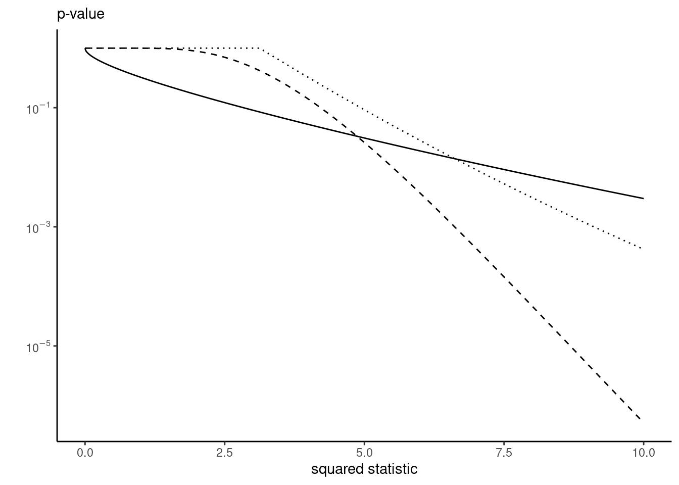
In R, we can use the multcomp or emmeans packages for the tests to adjust, or compute results manually. The test statistics do not change, only the benchmark null distribution is different. Figure 4.2 shows what the \(p\)-value would be depending on how we control for contrasts. For reasonable values, we get larger \(p\)-values for the methods that provide control.

Figure 4.2: P-value as a function of the squared t-statistic for a contrast for no adjustment (full line), Tukey’s HSD (dashed line) and Scheffe’s adjustment (dotted).

Example 4.4 (Multiple testing for paper or plastic) Sokolova, Krishna, and Döring (2023) considered pairwise difference relative to the control where only plastic wrapping is used. We could use either Bonferroni, Holm–Bonferoni or Dunnett’s method. Since the \(p\)-values are tiny (less than \(10^{-4}\)), this has no impact on the conclusions whatsoever. To better appreciate the impact in small samples, we subsample 20 observation per group to inflate \(p\)-values. We can also see differences by inspecting the width of the confidence intervals for the pairwise differences to the reference group: more conservative references lead to wider intervals.

data(SKD23_S2A, package = "hecedsm") # load data
set.seed(80667) # Set seed for reproducibility
SKD23_S2A_sub <- SKD23_S2A |>
  # Create a categorical variable (factor) and ensure reference is 0
  # By default, it would be (first alphanumerical value of labels)
  dplyr::mutate(propfact = relevel(factor(proportion), ref = "0")) |>
  # Sample only fourty observations by group -
  # for illustration purposes only, otherwise p-values are too small
  dplyr::slice_sample(n = 20, by = propfact)
anovamod <- lm(pef ~ propfact, data = SKD23_S2A_sub) 
library(emmeans)
margmean <- emmeans(
  anovamod, # fitted model
  # 'specs': vector with names of factors to adjust for
  specs = "propfact") 
contrastlist <- list( # specify contrast vectors
  refvshalf = c(1, -1, 0, 0),
  refvsone =  c(1, 0, -1, 0),
  refvstwo =  c(1, 0, 0, -1))
contrasts <- margmean |> contrast(method = contrastlist)
# Bonferroni and Holm-Bonferroni adjustments
summary(contrasts, adjust = "bonferroni")

 contrast  estimate    SE df t.ratio p.value
 refvshalf   -0.450 0.331 76  -1.359  0.5346
 refvsone    -1.150 0.331 76  -3.473  0.0026
 refvstwo    -0.662 0.331 76  -2.001  0.1470

P value adjustment: bonferroni method for 3 tests 

summary(contrasts, adjust = "holm")

 contrast  estimate    SE df t.ratio p.value
 refvshalf   -0.450 0.331 76  -1.359  0.1782
 refvsone    -1.150 0.331 76  -3.473  0.0026
 refvstwo    -0.662 0.331 76  -2.001  0.0980

P value adjustment: holm method for 3 tests 

# Note that the p-values for the latter are equal or smaller

# Adjustments for ANOVA to get simultaneous statements
# Number of groups minus 1 for Scheffe (correct here)
# This 'rank' often needs to be manually specified in multi-way ANOVA
summary(contrasts, adjust = "scheffe", scheffe.rank = 3)

 contrast  estimate    SE df t.ratio p.value
 refvshalf   -0.450 0.331 76  -1.359  0.6070
 refvsone    -1.150 0.331 76  -3.473  0.0104
 refvstwo    -0.662 0.331 76  -2.001  0.2696

P value adjustment: scheffe method with rank 3 

# This would be the better option here
summary(contrasts, adjust = "dunnett")

 contrast  estimate    SE df t.ratio p.value
 refvshalf   -0.450 0.331 76  -1.359  0.3934
 refvsone    -1.150 0.331 76  -3.473  0.0025
 refvstwo    -0.662 0.331 76  -2.001  0.1260

P value adjustment: dunnettx method for 3 tests 

# The less you adjust for, the smaller the p-values
# For Tukey, use 'contrast(method = "pairwise")' instead

# Since we have a small number of pairwise comparisons
# We could use the less stringent of Holm-Bonferroni and Dunnett's
# The latter provides shorter intervals here.
contrasts |> confint(adjust = "dunnett")

 contrast  estimate    SE df lower.CL upper.CL
 refvshalf   -0.450 0.331 76    -1.25    0.348
 refvsone    -1.150 0.331 76    -1.95   -0.352
 refvstwo    -0.662 0.331 76    -1.46    0.135

Confidence level used: 0.95 
Conf-level adjustment: dunnettx method for 3 estimates 

contrasts |> confint(adjust = "holm")

 contrast  estimate    SE df lower.CL upper.CL
 refvshalf   -0.450 0.331 76    -1.26    0.361
 refvsone    -1.150 0.331 76    -1.96   -0.339
 refvstwo    -0.662 0.331 76    -1.47    0.148

Confidence level used: 0.95 
Conf-level adjustment: bonferroni method for 3 estimates 

We can see that more stringent adjustments lead to higher \(p\)-values and wider intervals.

If we wanted to perform tests for multiple variables, or for subgroups, we can obtain overall control by using a procedure in each subset with a lower \(\alpha\), and combining the overall errors afterwards. If the data arise from different independent samples, the tests are indeed independent.

Baumann, James F., Nancy Seifert-Kessell, and Leah A. Jones. 1992. “Effect of Think-Aloud Instruction on Elementary Students’ Comprehension Monitoring Abilities.” Journal of Reading Behavior 24 (2): 143–72. https://doi.org/10.1080/10862969209547770.

Nosek, Brian, Johanna Cohoon, Mallory Kidwell, and Jeffrey Spies. 2015. “Estimating the Reproducibility of Psychological Science.” Science 349 (6251). https://doi.org/10.1126/science.aac4716.

Sokolova, Tatiana, Aradhna Krishna, and Tim Döring. 2023. “Paper Meets Plastic: The Perceived Environmental Friendliness of Product Packaging.” Journal of Consumer Research 50 (3): 468–91. https://doi.org/10.1093/jcr/ucad008.

---

1. Should you ever need the formula, the standard error assuming subsample size of \(n_1, \ldots, n_K\) and a common variance \(\sigma^2\) is \(\sqrt{\mathsf{Va}(\widehat{C})}\), where \[\mathsf{Va}(\widehat{C}) = \widehat{\sigma}^2\left(\frac{c_1^2}{n_1} + \cdots + \frac{c_K^2}{n_K}\right).\]

2. The constraint \(c_1 + \cdots + c_K=0\) ensures that linear contrasts are orthogonal to the mean, which has weight \(c_i=n_i/n\) and for balanced samples \(c_i =1/n\).

3. These would be formulated at registration time, but for the sake of the argument we proceed as if they were.

4. This is the case if tests are based on different data, or if the contrasts considered are orthogonal under normality.

5. The second line holds with independent observations, the second follows from the use of Boole’s inequality and does not require independent tests.

6. By definition, the expected number of false positive (PFER) is \(\mathsf{E}(V) = \sum_{i=1}^m i \Pr(V=i) \geq \sum_{i=1}^m \Pr(V=i) = \Pr(V \geq 1)\), so larger than the probability of making at least type 1 error. Thus, any procedure that controls the per-family error rate (e.g., Bonferroni) also automatically bounds the familywise error rate.