6 Repeated measures
So far, all experiments we have considered can be classified as between-subject designs, meaning that each experimental unit was assigned to a single experimental (sub)-condition. In many instances, it may be possible to randomly assign multiple conditions to each experimental unit. For example, an individual coming to a lab to perform tasks in a virtual reality environment may be assigned to all treatments. There is an obvious benefit to doing so, as the participants can act as their own control group, leading to greater comparability among treatment conditions.
For example, consider a study performed at Tech3Lab that looks at the reaction time for people texting or talking on a cellphone while walking. We may wish to determine whether disengagement is slower for people texting, yet we may also postulate that some elderly people have slower reflexes.
By including multiple conditions, we can filter out the effect due to subject: this leads to increased precision of effect sizes and increased power (as we will see, hypothesis tests are based on within-subject variability). Together, this translates into the need to gather fewer observations or participants to detect a given effect in the population and thus experiments are cheaper to run.
There are of course drawbacks to gathering repeated measures from individuals. Because subjects are confronted with multiple tasks, there may be carryover effects (when one task influences the response of the subsequent ones, for example becoming better as manipulations go on), period effects (fatigue, a decrease in acuity), and permanent changes in the subject condition after a treatment or attrition (loss of subjects over time).
To minimize potential biases, there are multiple strategies one can use. Tasks are normally presented in random order among subjects to avoid confounding, or using a balanced crossover design and include the period and carryover effect in the statistical model via control variables so as to better isolate the treatment effect. The experimenter should also allow enough time between treatment conditions to reduce or eliminate period or carryover effects and plan tasks accordingly.
If each subject is assigned to an experimental condition only once, one good way to do this is via counterbalancing. We proceed as follows: first, enumerate all possible orders of the condition and then assign participants as equally as possible between conditions. For example, with a single within-factor design with three conditions \(A, B, C\), we have six possible orderings (either \(ABC\), \(ACB\), \(BAC\), \(BCA\), \(CAB\) or \(CBA\)). Much like other forms of randomization, this helps us remove confounding effects and let’s us estimate what is the average effect of task ordering on the response.
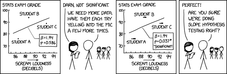
There are multiple approaches to handling repeated measures. The first option is to take averages over experimental condition per subject and treat them as additional blocking factors, but it may be necessary to adjust the resulting statistics. The second approach consists in fitting a multivariate model for the response and explicitly account for the correlation, otherwise the null distribution commonly used are off and so are the conclusions, as illustrated with the absurd comic displayed in Figure 13.1.
6.1 Repeated measures
We introduce the concept of repeated measure and within-subject ANOVA with an example.
Example 6.1 (Happy fakes) We consider an experiment conducted in a graduate course at HEC, Information Technologies and Neuroscience, in which PhD students gathered electroencephalography (EEG) data. The project focused on human perception of deepfake image created by a generative adversarial network: Amirabdolahian and Ali-Adeeb (2021) expected the attitude towards real and computer generated image of people smiling to change.
The response variable is the amplitude of a brain signal measured at 170 ms after the participant has been exposed to different faces. Repeated measures were collected on 9 participants given in the database AA21, who were expected to look at 120 faces. Not all participants completed the full trial, as can be checked by looking at the cross-tabs of the counts
data(AA21, package = "hecedsm")
xtabs(~stimulus + id, data = AA21)
id
stimulus 1 2 3 4 5 6 7 8 9 10 11 12
real 30 32 34 32 38 29 36 36 40 30 39 33
GAN1 32 31 40 33 38 29 39 31 39 28 35 34
GAN2 31 33 37 34 38 29 34 36 40 33 35 32The experimental manipulation is encoded in the stimuli, with levels control (real) for real facial images, whereas the others were generated using a generative adversarial network (GAN) with be slightly smiling (GAN1) or extremely smiling (GAN2); the latter looks more fake. While the presentation order was randomized, the order of presentation of the faces within each type is recorded using the epoch variable: this allows us to measure the fatigue effect.
Since our research question is whether images generated from generative adversarial networks trigger different reactions, we will be looking at pairwise differences with the control.
We could first grouping the data and compute the average for each experimental condition stimulus per participant and set id as blocking factor. The analysis of variance table obtained from aov would be correct, but would fail to account for correlation.
The one-way analysis of variance with \(n_s\) subjects, each of which was exposed to the \(n_a\) experimental conditions, can be written \[\begin{align*}\underset{\text{response}\vphantom{l}}{Y_{ij}} = \underset{\text{global mean}}{\mu_{\vphantom{j}}} + \underset{\text{mean difference}}{\alpha_j} + \underset{\text{subject difference}}{s_{i\vphantom{j}}} + \underset{\text{error}\vphantom{l}}{\varepsilon_{ij}} \end{align*}\]
# Compute mean for each subject +
# experimental condition subgroup
AA21_m <- AA21 |>
  dplyr::group_by(id, stimulus) |>
  dplyr::summarize(latency = mean(latency))
# Use aov for balanced sample
fixedmod <- aov(
  latency ~ stimulus + Error(id/stimulus),
  data = AA21_m)
# Print ANOVA table
summary(fixedmod)
Error: id
          Df Sum Sq Mean Sq F value Pr(>F)
Residuals 11  187.8   17.07

Error: id:stimulus
          Df Sum Sq Mean Sq F value Pr(>F)
stimulus   2   1.94  0.9704   0.496  0.615
Residuals 22  43.03  1.9557
Since the design is balanced after averaging, we can use aov in R: we need to specify the subject identifier within Error term. This approach has a drawback, as variance components can be negative if the variability due to subject is negligible. While aov is fast, it only works for simple balanced designs.
6.1.1 Contrasts
With balanced data, the estimated marginal means coincide with the row averages. If we have a single replication or the average for each subject/condition, we could create a new column with the contrast and then fit a model with an intercept-only (global mean) to check whether the latter is zero. With 12 participants, we should thus expect our test statistic to have 11 degrees of freedom, since one unit is spent on estimating the mean parameter and we have 12 participants.
Unfortunately, the emmeans package analysis for object fitted using aov will be incorrect: this can be seen by passing a contrast vector and inspecting the degrees of freedom. The afex package includes functionalities that are tailored for within-subject and between-subjects and has an interface with emmeans.
afexmod <- afex::aov_ez(
  id = "id",           # subject id
  dv = "latency",      # response variable
  within = "stimulus", # within-subject factor
  data = AA21,
  fun_aggregate = mean)
The afex package has different functions for computing the within-subjects design and the aov_ez specification, which allow people to list within and between-subjects factor separately with subject identifiers may be easier to understand. It also has an argument, fun_aggregate, to automatically average replications.
# Set up contrast vector
cont_vec <- list(
  "real vs GAN" = c(1, -0.5, -0.5))
library(emmeans)
# Correct output
afexmod |>
  emmeans::emmeans(
    spec = "stimulus",
    contr = cont_vec)
$emmeans
stimulus emmean SE df lower.CL upper.CL
real -10.8 0.942 11 -12.8 -8.70
GAN1 -10.8 0.651 11 -12.3 -9.40
GAN2 -10.3 0.662 11 -11.8 -8.85
Confidence level used: 0.95
$contrasts
contrast estimate SE df t.ratio p.value
real vs GAN -0.202 0.552 11 -0.366 0.7213# Incorrect output -
# note the wrong degrees of freedom
fixedmod |>
emmeans::emmeans(
spec = "stimulus",
contr = cont_vec)Note: re-fitting model with sum-to-zero contrasts$emmeans
stimulus emmean SE df lower.CL upper.CL
real -10.8 0.763 16.2 -12.4 -9.15
GAN1 -10.8 0.763 16.2 -12.4 -9.21
GAN2 -10.3 0.763 16.2 -11.9 -8.69
Warning: EMMs are biased unless design is perfectly balanced
Confidence level used: 0.95
$contrasts
contrast estimate SE df t.ratio p.value
real vs GAN -0.202 0.494 22 -0.409 0.68676.1.2 Sphericity assumption
The validity of the \(F\) statistic null distribution relies on the model having the correct structure.
In repeated-measure analysis of variance, we assume again that each measurement has the same variance. We equally require the correlation between measurements of the same subject to be the same, an assumption that corresponds to the so-called compound symmetry model.1
What if the within-subject measurements have unequal variance or the correlation between those responses differs?
Since we care only about differences in treatment, can get away with a weaker assumption than compound symmetry (equicorrelation) by relying instead on sphericity, which holds if the variance of the difference between treatment is constant. Sphericity is not a relevant concept when there is only two measurements (as there is a single correlation); we could check this by comparing the fit of a model with an unstructured covariance (difference variances for each and correlations for each pair of variable)
The most popular approach to handling correlation in tests is a two-stage approach: first, check for sphericity (using, e.g., Mauchly’s test of sphericity). If the null hypothesis of sphericity is rejected, one can use a correction for the \(F\) statistic by modifying the parameters of the Fisher \(\mathsf{F}\) null distribution used as benchmark.
An idea due to Box is to correct the degrees of freedom of the \(\mathsf{F}(\nu_1, \nu_2)\) distribution by multiplying them by a common factor \(\epsilon<1\) and use \(\mathsf{F}(\epsilon\nu_1, \epsilon\nu_2)\) as null distribution instead to benchmark our statistics and determine how extreme our observed one is. Since the \(F\) statistic is a ratio of variances, the \(\epsilon\) terms would cancel. Using the scaled \(\mathsf{F}\) distribution leads to larger \(p\)-values, thus accounting for the correlation.
There are three widely used corrections: Greenhouse–Geisser, Huynh–Feldt and Box correction, which divides by \(\nu_1\) both degrees of freedom and gives a very conservative option. The Huynh–Feldt method is reported to be more powerful so should be preferred, but the estimated value of \(\epsilon\) can be larger than 1.
Using the afex functions, we get the result for Mauchly’s test of sphericity and the \(p\) values from using either correction method
summary(afexmod)
Univariate Type III Repeated-Measures ANOVA Assuming Sphericity

            Sum Sq num Df Error SS den Df  F value    Pr(>F)
(Intercept) 4073.1      1  187.814     11 238.5554 8.373e-09 ***
stimulus       1.9      2   43.026     22   0.4962    0.6155
---
Signif. codes:  0 '***' 0.001 '**' 0.01 '*' 0.05 '.' 0.1 ' ' 1


Mauchly Tests for Sphericity

         Test statistic p-value
stimulus        0.67814 0.14341


Greenhouse-Geisser and Huynh-Feldt Corrections
 for Departure from Sphericity

          GG eps Pr(>F[GG])
stimulus 0.75651     0.5667

            HF eps Pr(>F[HF])
stimulus 0.8514944  0.5872648
Example 6.2 (Enjoyment from waiting) We consider Experiment 3 from Hatano et al. (2022). The data consist in a two by two mixed analysis of variance. The authors studied engagement and enjoyment from waiting tasks, and “potential effects of time interval on the underestimation of task motivation by manipulating the time for the waiting task”. The waiting time was randomly assigned to either short (3 minutes) or long (20 minutes) with equal probability, but participants were either told that there was a 70% chance of being assigned to the short session, or 30% chance. We first load the data from the package and inspect the content.
tibble [126 × 4] (S3: tbl_df/tbl/data.frame)
 $ id        : Factor w/ 63 levels "1","2","3","4",..: 1 1 2 2 3 3 4 4 5 5 ...
 $ waiting   : Factor w/ 2 levels "long","short": 2 2 1 1 1 1 2 2 1 1 ...
 $ ratingtype: Factor w/ 2 levels "experience","prediction": 2 1 2 1 2 1 2 1 2 1 ...
 $ imscore   : num [1:126] 2.33 3.33 1.25 1.92 1 ...
waiting
long short
32 31 From this, we can see that there each student is assigned to a single waiting time, but that they have both rating types. Since there are 63 students, the study is unbalanced but by a single person; this may be due to exclusion criteria. We use the afex package (analysis of factorial design) with the aov_ez function to fit the model in R. We need to specify the identifier of the subjects (id), the response variable (dv) and both between- (between) and within-subject (within) factors. Each of those names must be quoted.
Anova Table (Type 3 tests)

Response: imscore
                   num Df den Df     MSE       F      ges    Pr(>F)
waiting                 1     61 2.48926 11.2551 0.126246   0.00137 **
ratingtype              1     61 0.68953 38.4330 0.120236 5.388e-08 ***
waiting:ratingtype      1     61 0.68953  0.0819 0.000291   0.77575
---
Signif. codes:  0 '***' 0.001 '**' 0.01 '*' 0.05 '.' 0.1 ' ' 1
The output includes the \(F\)-tests for the two main effects and the interaction and global effect sizes \(\widehat{\eta}^2\) (ges). There is no output for tests of sphericity, since there are only two measurements per person and thus a single mean different within-subject (so the test to check equality doesn’t make sense with a single number). We could however compare variance between groups using Levene’s test. Note that the degrees of freedom for the denominator of the test are based on the number of participants, here 63.
Note that, with two measurements, there is a single correlation parameter to estimate and this assumption is irrelevant.↩︎