8 Multivariate analysis of variance
Multivariate analysis of variance (MANOVA) leads to procedures that are analogous to univariate analysis of variance, but we now need to estimate correlation and variance parameters for each measurement separately and there are multiple potential statistics that can be defined for testing effects. While we can benefit from the correlation and find differences that wouldn’t be detected from univariate models, the additional parameters to estimate lead to a loss of power. Finally, the most popular method nowadays for handling repeated measures is to fit a mixed model, with random effects accounting to subject-specific characteristics. By doing so, we assume that the levels of a factor (here the subject identifiers) form a random sample from a large population. These models can be difficult to fit and one needs to take great care in specifying the model.
The second paradigm for modelling is to specify that the response from each subject is in fact a multivariate object: we can combine all measurements from a given individual in a vector \(\boldsymbol{Y}\). In the example with the happy fakes, this would be the tuple of measurements for (real, GAN1, GAN2).
The multivariate analysis of variance model is designed by assuming observations follow a (multivariate) normal distribution with mean vector \(\boldsymbol{\mu}_j\) in group \(j\) and common covariance matrix \(\boldsymbol{\Sigma}\) and comparing means between groups. As in univariate analysis of variance, the multivariate normal assumption holds approximately by virtue of the central limit theorem in large samples, but the convergence is slower and larger numbers are needed to ensure this is valid.
The difference with the univariate approach is now that we will compare a global mean vector \(\boldsymbol{\mu}\) between comparisons. In the one-way analysis of variance model with an experimental factor having \(K\) levels and a balanced sample \(n_g\) observations per group and \(n=n_gK\) total observations, we assume that each group has average \(\boldsymbol{\mu}_k\) \((k=1, \ldots, K)\), which we can estimate using only the observations from that group. Under the null hypothesis, all groups have the same mean, so the estimator is the overall mean \(\boldsymbol{\mu}\) combining all \(n\) observations.
The statistic is obtained by decomposing the total variance around the global mean into components due to the different factors and the leftover variability. Because these equivalent to the sum of square decomposition results in multiple matrices, there are multiple ways of constructing test statistics. Wilk’s \(\Lambda\) is the most popular choice. Another common choice, which leads to a statistic giving lower power but which is also more robust to departure from model assumptions is Pillai’s trace.
The MANOVA model assumes that the covariance matrices are the same within each experimental condition. We can use Box’s \(M\) statistic to test the normality hypothesis.
8.1 Data format
With repeated measures, it is sometimes convenient to store measurements associated to each experimental condition in different columns of a data frame or spreadsheet, with lines containing participants identifiers. Such data are said to be in wide format, since there are multiple measurements in each row. While this format is suitable for storate, many statistical routines will instead expect data to be in long format, for which there is a single measurement per line. Figure 8.1 illustrates the difference between the two formats.
Ideally, a data base in long format with repeated measures would also include a column giving the order in which the treatments were assigned to participants. This is necessary in order to test whether there are fatigue or crossover effects, for example by plotting the residuals after accounting for treatment subject by subject, ordered over time. We could also perform formal tests by including time trends in the model and checking whether the slope is significant.
Overall, the biggest difference with within-subject designs is that observations are correlated whereas we assumed measurements were independent until now. This needs to be explicitly accounted for, as correlation has an important impact on testing as discussed Section 3.4.4: failing to account for correlation leads to \(p\)-values that are much too low. To see why, think about a stupid setting under which we duplicate every observation in the database: the estimated marginal means will be the same, but the variance will be halved despite the fact there is no additional information. Intuitively, correlation reduces the amount of information provided by each individual: if we have repeated measures from participants, we expect the effective sample size to be anywhere between the total number of subjects and the total number of observations.
8.2 Mathematical complement
This section is technical and can be omitted. Analogous to the univariate case, we can decompose the variance estimator in terms of within, between and total variance. Let \(\boldsymbol{Y}_{ik}\) denote the response vector for the \(i\)th observation of group \(k\); then, we can decompose the variance as \[\begin{align*} & \underset{\text{total variance}}{\sum_{k=1}^K \sum_{i=1}^{n_g} (\boldsymbol{Y}_{ik} - \widehat{\boldsymbol{\mu}})(\boldsymbol{Y}_{ik} - \widehat{\boldsymbol{\mu}})^\top} \\\qquad &= \underset{\text{within variance}}{\sum_{k=1}^K \sum_{i=1}^{n_g} (\boldsymbol{Y}_{ik} - \widehat{\boldsymbol{\mu}}_k)(\boldsymbol{Y}_{ik} - \widehat{\boldsymbol{\mu}}_k)^\top} + \underset{\text{between variance}}{\sum_{k=1}^K n_g(\boldsymbol{\mu}_{k} - \widehat{\boldsymbol{\mu}})(\widehat{\boldsymbol{\mu}}_k - \widehat{\boldsymbol{\mu}})^\top} \end{align*}\] defining covariance matrix estimators. If we write \(\widehat{\boldsymbol{\Sigma}}_T,\) \(\widehat{\boldsymbol{\Sigma}}_W\), and \(\widehat{\boldsymbol{\Sigma}}_B\) for respectively the total, within and between variance estimators, we can build a statistic from these ingredients to see how much variability is induced by centering using a common vector. When \(K>2\), there are multiple statistics that be constructed, including
- Wilk’s \(\Lambda\): \(|\widehat{\boldsymbol{\Sigma}}_W|/|\widehat{\boldsymbol{\Sigma}}_W + \widehat{\boldsymbol{\Sigma}}_B|\)
- Roy’s maximum root: the largest eigenvalue of \(\widehat{\boldsymbol{\Sigma}}_W^{-1}\widehat{\boldsymbol{\Sigma}}_B\)
- Lawley–Hotelling trace: \(\mathrm{tr}(\widehat{\boldsymbol{\Sigma}}_W^{-1}\widehat{\boldsymbol{\Sigma}}_B)\)
- Pillai’s trace: \(\mathrm{tr}\left\{\widehat{\boldsymbol{\Sigma}}_B(\widehat{\boldsymbol{\Sigma}}_W +\widehat{\boldsymbol{\Sigma}}_B)^{-1}\right\}\).
All four criteria lead to equivalent statistics and the same \(p\)-values if \(K=2\).
With a two-way balanced MANOVA, we can perform a similar decomposition for each factor or interaction, with \[\widehat{\boldsymbol{\Sigma}}_T = \widehat{\boldsymbol{\Sigma}}_A + \widehat{\boldsymbol{\Sigma}}_B + \widehat{\boldsymbol{\Sigma}}_{AB} + \widehat{\boldsymbol{\Sigma}}_W.\]
Wilk’s \(\Lambda\) is based on taking the ratio of the determinant of the within-variance and that of the sum of effect-variance plus within-variance, e.g., \(|\widehat{\boldsymbol{\Sigma}}_{AB} + \widehat{\boldsymbol{\Sigma}}_W|\) for the interaction term.
8.3 Model fitting
We can treat the within-subject responses as a vector of observations and estimate the model using using multivariate linear regression. Contrary to the univariate counterpart, the model explicitly models the correlation between observations from the same subject.
In order to fit a model with a multivariate response, we first need to pivot the data into wider format so as to have a matrix with rows for the number of subjects and \(M\) columns for the number of response variables.
Once the data are in a suitable format, we fit the multivariate model with the lm function using the sum-to-zero constraints, here imposed globally by changing the contrasts option. Syntax-wise, the only difference with the univariate case is that the response on the left of the tilde sign (~) is now a matrix composed by binding together the vectors with the different responses.
Example 8.1 (A multivariate take on “Happy fakes”) We use the data from Amirabdolahian and Ali-Adeeb (2021), but this time treating the averaged repeated measures for the different stimulus as a multivariate response. We first pivot the data to wide format, then fit the multivariate linear model.
data(AA21, package = "hecedsm")
# Compute mean per subject
AA21_m <- AA21 |>
  dplyr::group_by(id, stimulus) |>
  dplyr::summarize(latency = mean(latency))
`summarise()` has grouped output by 'id'. You can override using the `.groups`
argument.# Pivot to wide format (one individual, multiple measurements per line)
AA21_mw <- AA21_m |>
tidyr::pivot_wider(names_from = stimulus, # within-subject factor labels
values_from = latency) # response measurements
# Model with each variable with a different mean
# Specify all columns with column bind
# left of the ~, following
options(contrasts = c("contr.sum", "contr.poly"))
mlm <- lm(cbind(real, GAN1, GAN2) ~ 1,
data = AA21_mw)Since the within-subject factor stimulus disappeared when we consider the multivariate response, we only specify a global mean vector \(\boldsymbol{\mu}\) via ~1. In general, we would add the between-subject factors to the right-hand side of the equation. Our hypothesis of equal mean translates into the hypothesis \(\boldsymbol{\mu} = \mu\boldsymbol{1}_3\), which can be imposed using a call to anova. The output returns the statistic and \(p\)-values including corrections for sphericity.
We can also use emmeans to set up post-hoc contrasts. Since we have no variable, we need to set in specs the repeated measure variable appearing on the left hand side of the formula; the latter is labelled rep.meas by default.
# Test the multivariate model against
# equal mean (X = ~1)
anova(mlm, X = ~1, test = "Spherical")
Analysis of Variance Table
Contrasts orthogonal to
~1
Greenhouse-Geisser epsilon: 0.7565
Huynh-Feldt epsilon: 0.8515
Df F num Df den Df Pr(>F) G-G Pr H-F Pr
(Intercept) 1 0.4962 2 22 0.61549 0.56666 0.58726
Residuals 11 # Follow-up contrast comparisons
library(emmeans)
emm_mlm <- emmeans(mlm, specs = "rep.meas")
emm_mlm |> contrast(method = list(c(1,-0.5,-0.5))) contrast estimate SE df t.ratio p.value
c(1, -0.5, -0.5) -0.202 0.552 11 -0.366 0.7213We can check that the output is the same in this case as the within-subject analysis of variance model fitted previously with the afex package.
Example 8.2 (Teaching to read) We consider a between-subject repeated measure multivariate analysis of variance model with the Baumann, Seifert-Kessell, and Jones (1992). The data are balanced by experimental condition and they include the results of three tests performed after the intervention: an error detection task, an expanded comprehension monitoring questionnaire and a cloze test. Note that the scale of the tests are different (16, 18 and 56).
We could obtain the estimated covariance matrix of the fitted model by extracting the residuals \(Y_{ik} - \widehat{\mu}_k\) and computing the empirical covariance. The results shows a strong dependence between tests 1 and 3 (correlation of 0.39), but much weaker dependence with test 2.
Let us compute the multivariate analysis of variance model
data(BSJ92, package = "hecedsm")
# Force sum-to-zero parametrization
options(contrasts = c("contr.sum", "contr.poly"))
# Fit MANOVA model
mmod <- lm(
  cbind(posttest1, posttest2, posttest3) ~ group,
   data = BSJ92)
# Calculate multivariate test
mtest <- car::Anova(mmod, test = "Wilks")
# mtest
# Get all statistics and univariate tests
summary(car::Anova(mmod), univariate = TRUE)
Type II MANOVA Tests:

Sum of squares and products for error:
          posttest1  posttest2 posttest3
posttest1 640.50000   30.77273  498.3182
posttest2  30.77273  356.40909 -104.3636
posttest3 498.31818 -104.36364 2511.6818

------------------------------------------

Term: group

Sum of squares and products for the hypothesis:
           posttest1 posttest2 posttest3
posttest1 108.121212  6.666667 190.60606
posttest2   6.666667 95.121212  56.65152
posttest3 190.606061 56.651515 357.30303

Multivariate Tests: group
                 Df test stat approx F num Df den Df     Pr(>F)
Pillai            2 0.4082468 5.300509      6    124 6.7654e-05 ***
Wilks             2 0.6320200 5.243287      6    122 7.7744e-05 ***
Hotelling-Lawley  2 0.5185169 5.185169      6    120 8.9490e-05 ***
Roy               2 0.3184494 6.581288      3     62 0.00062058 ***
---
Signif. codes:  0 '***' 0.001 '**' 0.01 '*' 0.05 '.' 0.1 ' ' 1

 Type II Sums of Squares
          df posttest1 posttest2 posttest3
group      2    108.12    95.121     357.3
residuals 63    640.50   356.409    2511.7

 F-tests
      posttest1 posttest2 posttest3
group      5.32      8.41      4.48

 p-values
      posttest1  posttest2  posttest3
group 0.00734676 0.00058043 0.01515115
By default, we get Pillai’s trace statistic. Here, there is clear evidence of differences between groups of observations regardless of the statistic being used.
We can compute effect size as before by passing the table, for example using eta_squared(mtest) to get the effect size of the multivariate test, or simple the model to get the individual variable effect sizes.
Having found a difference, one could in principle investigate for which component of the response they are by performing univariate analysis of variance and accounting for multiple testing using, e.g., Bonferroni’s correction. A more fruitful avenue if you are trying to discriminate is to use descriptive discriminant analysis as a follow-up, which computes the best fitting hyperplanes that separate groups.
MASS::lda(group ~ posttest1 + posttest2 + posttest3,
          data = BSJ92)
This amounts to compute the weights \(\boldsymbol{w}\) such, that, computing \(\boldsymbol{w}^\top\boldsymbol{Y}\) creating a composite score by adding up weighted components that leads to maximal separation between groups. Figure 8.2 shows the new coordinates.
Linear discriminant analysis is a topic on it’s own that is beyond the scope of the course.
8.4 Model assumptions
In addition to the usual model assumptions (independence of measurements from different subjects, equal variance, additivity, etc.), the MANOVA model adds two hypothesis that altogether determine how reliable our \(p\)-values and conclusions are.
The first assumption is that of multivariate normality of the response. The central limit theorem can be applied to a multivariate response, but the sample size needed overall to reliably estimate the correlation and variance is larger than in the univariate setting. This hypothesis can be tested using the Shapiro-Wilk normality test (null hypothesis is that of normality) by passing the residuals of the multivariate model. Such a test can lead to rejection of the null hypothesis when specific variables are far from normal, or when the dependence structure isn’t the one exhibited by a multivariate normal model. With decent sample sizes (say \(n=50\) per group), this assumption isn’t as important as others.
# Shapiro-Wilk normality test
# Must transpose the residuals
# to get a 3 by n matrix
mvnormtest::mshapiro.test(U = t(resid(mmod)))
    Shapiro-Wilk normality test

data:  Z
W = 0.96464, p-value = 0.05678
The second assumption is that the covariance matrix is the same for all individuals, regardless of their experimental group assignment. We could try checking whether a covariance model in each group: under multivariate normal assumption, this leads to a test statistic called Box’s \(M\) test. Unfortunately, this test is quite sensitive to departures from the multivariate normal assumption and, if the \(p\)-value is small, it may have to do more with the normality than the heterogeneity.
with(BSJ92,
     biotools::boxM(
       data = cbind(posttest1, posttest2, posttest3),
       grouping = group))
    Box's M-test for Homogeneity of Covariance Matrices

data:  cbind(posttest1, posttest2, posttest3)
Chi-Sq (approx.) = 15.325, df = 12, p-value = 0.2241
In our example, there is limited evidence against any of those model assumptions. We should of course also check the assumptions of the analysis of variance model for each of postest1, posttest2 and posttest3 in turn; such a check is left as an exercice to the reader.
8.5 Power and effect size
Since all of the multivariate statistics can be transformed for a comparison with a univariate \(\mathsf{F}\) distribution, we can estimate partial effect size as before. The package effectsize offers a measure of partial \(\widehat{\eta}^2\) for the multivariate tests.1
Power calculations are beyond the reach of ordinary software as one needs to specify the variance of each observation, their correlation and their mean. Simulation is an obvious way for this kind of design to obtain answers, but the free G\({}^{*}\)Power software (Faul et al. 2007) also offers some tools. See also Läuter (1978) for pairwise comparisons: to achieve a power of 80%, we need the following number of replicates per group \(j=1, \ldots, J\), which shows that the number increases rapidly with the dimension of the response vector \(p\). As usual, smaller effect sizes are more difficult to detect.
3 groups
|
4 groups
|
5 groups
|
||||||||||
|---|---|---|---|---|---|---|---|---|---|---|---|---|
| effect size \ p | 2 | 4 | 6 | 8 | 2 | 4 | 6 | 8 | 2 | 4 | 6 | 8 |
| very large | 13 | 16 | 18 | 21 | 14 | 18 | 21 | 23 | 16 | 21 | 24 | 27 |
| large | 26 | 33 | 38 | 42 | 29 | 37 | 44 | 48 | 34 | 44 | 52 | 58 |
| medium | 44 | 56 | 66 | 72 | 50 | 64 | 74 | 84 | 60 | 76 | 90 | 100 |
| small | 98 | 125 | 145 | 160 | 115 | 145 | 165 | 185 | 135 | 170 | 200 | 230 |
Example 8.3 (Disclosure formats for companies) The data presented in this example vignette is inspired by a study from Anandarajan, Viger, and Curatola (2002), who looked at the impact of communication means through different disclosure format on the perceived risk of organization on the brink of bankruptcy in accountancy. There is a single between-subject factor for the disclore format, and three measures of the performance, ratings for the interest rate premium assessed, for the ability to service debt and that to improve profitability. We first load the data from the package and inspect the content.
data(AVC02, package = "hecedsm")
str(AVC02)
tibble [132 × 4] (S3: tbl_df/tbl/data.frame)
$ format : Factor w/ 3 levels "integrated note",..: 1 1 1 1 1 1 1 1 1 1 ...
$ prime : num [1:132] 0.5 1.5 0.5 0.25 1.5 1.25 2 0.5 1.5 0.5 ...
$ debt : int [1:132] 3 4 1 4 3 3 3 5 2 2 ...
$ profitability: int [1:132] 3 2 2 5 2 2 2 3 2 3 ...xtabs(~ format, data = AVC02)format
integrated note stand-alone note modified auditor report
40 45 47 The data are unbalanced by condition. In general, we need them to be roughly balanced to maximize power. The manova function will not be usable unless data are balanced, and we need to enforce sum-to-zero constraints to get sensible outputs. After this is done, we can fit the multivariate linear model with lm by binding columns on the left of the ~ sign to gather the response vectors.
options(contrasts = c("contr.sum", "contr.poly"))
model <- lm(cbind(prime, debt, profitability) ~ format,
            data = AVC02)
We can check the residual correlation matrix to see if there was a strong dependence between our measurements. The benefit of MANOVA is to be able to leverage this correlation, if any.
cor(resid(model)) prime debt profitability
prime 1.00 -0.40 -0.54
debt -0.40 1.00 0.65
profitability -0.54 0.65 1.00We can look at the global mean for each variable and the estimated mean differences for all groups, including the reference which is omitted. It’s easy to see that the mean differences sum to zero.
dummy.coef(model)Full coefficients are
(Intercept): prime 1.280511
debt 2.881521
profitability 2.597695
format: integrated note stand-alone note
prime -0.099261229 -0.013844563
debt 0.068479117 -0.059298660
profitability 0.127304965 0.002304965
(Intercept):
format: modified auditor report
0.113105792
-0.009180457
-0.129609929Next, we compute the multivariate analysis of variance table and the follow-up with the univariate functions. By default, we can add a multiplicity correction for the tests, using Holm-Bonferonni with option 'holm'. For the MANOVA test, there are multiple statistics to pick from, including Pillai, Wilks, Hotelling-Lawley and Roy. The default is Pillai, which is more robust to departures from the model hypothesis, but Wilks is also popular choice among practitioners.
car::Manova(model, test = "Pillai")
Type II MANOVA Tests: Pillai test statistic
       Df test stat approx F num Df den Df Pr(>F)
format  2   0.02581  0.55782      6    256 0.7637
We can compute effect sizes overall for the MANOVA statistic using the correspondance with the \(F\) distribution, and also the individual effect size variable per variable. Here, the values returned are partial \(\widehat{\eta}^2\) measures.
effectsize::eta_squared(car::Manova(model))# Effect Size for ANOVA (Type II)
Parameter | Eta2 (partial) | 95% CI
-----------------------------------------
format | 0.01 | [0.00, 1.00]
- One-sided CIs: upper bound fixed at [1.00].# Since it's a one-way between-subject MANOVA, no partial measure
effectsize::eta_squared(model, partial = FALSE)# Effect Size for ANOVA (Type I)
Response | Parameter | Eta2 | 95% CI
---------------------------------------------------
prime | format | 0.01 | [0.00, 1.00]
debt | format | 2.23e-03 | [0.00, 1.00]
profitability | format | 0.02 | [0.00, 1.00]We can continue with descriptive discriminant analysis for the post-hoc comparisons. To fit the model using the lda function from the MASS package, we swap the role of the experimental factor and responses in the formula. The output shows the weights for the linear combinations.
MASS::lda(format ~ prime + debt + profitability,
          data = AVC02)
Call:
lda(format ~ prime + debt + profitability, data = AVC02)
Prior probabilities of groups:
integrated note stand-alone note modified auditor report
0.3030303 0.3409091 0.3560606
Group means:
prime debt profitability
integrated note 1.181250 2.950000 2.725000
stand-alone note 1.266667 2.822222 2.600000
modified auditor report 1.393617 2.872340 2.468085
Coefficients of linear discriminants:
LD1 LD2
prime 0.5171202 0.16521149
debt 0.6529450 0.97286350
profitability -1.2016530 -0.04412713
Proportion of trace:
LD1 LD2
0.9257 0.0743 Interpretation of these is beyond the scope of the course, but you can find information about linear discriminant analysis in good textbooks (e.g., Chapter 12 of Mardia, Kent, and Taylor 2024). The next step before writing about any of our conclusions is to check the model assumptions. As before, we could check for each variable in turn whether the variance are the same in each group. Here, we rather check equality of covariance matrix. The test has typically limited power, but unfortunately is very sensitive to departure from the multivariate normality assumption, so sometimes rejections are simply due to false positive.
with(AVC02,
biotools::boxM(cbind(prime, debt, profitability),
               grouping = format))
    Box's M-test for Homogeneity of Covariance Matrices

data:  cbind(prime, debt, profitability)
Chi-Sq (approx.) = 21.274, df = 12, p-value = 0.0465
We get a smallish \(p\)-value, and therefore weak evidence against equality of covariance matrices. The data were generated from normal distribution, so the small \(p\)-value is likely an artifact of the rounding of the Likert scale. We can test the normality assumption using univariate quantile-quantile plots or tests of normality, including Shapiro-Wilks.
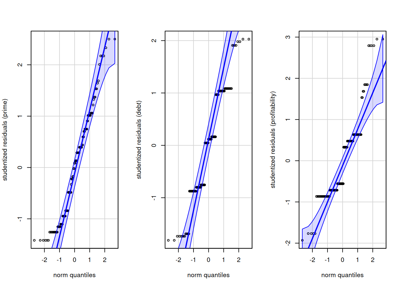
We see severe rounding impacts for debt and profitability. There is little to be done about this, but the sample size are large enough that this shouldn’t be too much a concern. We can also test the multivariate normality assumption. The latter supposes that observations in each group have the same mean. To get this, we detrend using multivariate linear model by subtracting the mean of each group. Thus, our input is the matrix of residuals, which must be transposed for the function to work.
mvnormtest::mshapiro.test(U = t(resid(model)))
    Shapiro-Wilk normality test

data:  Z
W = 0.96982, p-value = 0.004899
There is (unsurprisingly) strong evidence against multivariate normality, but it matters less due to sample size. This is a consequence of the discrete univariate measurements, which explain rejection of the null (for data to be multivariate normal, each of the response must be univariate normal and the dependence structure must also match. Since model assumptions are doubtful, we recommend using Pilai’s trace as test statistic for the MANOVA.
I must confess I haven’t checked whether the output is sensical.↩︎