2  Hypothesis testing

In most applied domains, empirical evidences drive the advancement of the field and data from well designed experiments contribute to the built up of science. In order to draw conclusions in favour or against a theory, researchers turn (often unwillingly) to statistics to back up their claims. This has led to the prevalence of the use of the null hypothesis statistical testing (NHST) framework. One important aspect of the reproducibility crisis is the misuse of \(p\)-values in journal articles: falsification of a null hypothesis is not enough to provide substantive findings for a theory.

Because introductory statistics course typically present hypothesis tests without giving much thoughts to the underlying construction principles of such procedures, users often have a reductive view of statistics as a catalogue of pre-determined procedures. To make a culinary analogy, users focus on learning recipes rather than trying to understand the basics of cookery. This chapter focuses on understanding of key ideas related to testing.

Key concept

Learning objectives:

• Understanding the role of uncertainty in decision making.
• Understanding the importance of signal-to-noise ratio as a measure of evidence.
• Knowing the basic ingredients of hypothesis testing and being capable of correctly formulating and identifying these components in a paper.
• Correctly interpreting \(p\)-values and confidence intervals for a parameter.

2.1 Hypothesis

The first step of a design is formulating a research question. Generally, this hypothesis will specify potential differences between population characteristics due to some intervention (a treatment) that the researcher wants to quantify. This is the step during which researchers decide on sample size, choice of response variable and metric for the measurement, write down the study plan, etc.

It is important to note that most research questions cannot be answered by simple tools. Researchers wishing to perform innovative methodological research should contact experts and consult with statisticians before they collect their data to get information on how best to proceed for what they have in mind so as to avoid the risk of making misleading and false claims based on incorrect analysis or data collection.

Figure 2.1: xkcd comic 2569 (Hypothesis generation) by Randall Munroe. Alt text: Frazzled scientists are requesting that everyone please stop generating hypotheses for a little bit while they work through the backlog. Cartoon reprinted under the CC BY-NC 2.5 license.

2.2 Sampling variability

Given data, a researcher will be interested in estimating particular characteristics of the population. We can characterize the set of all potential values their measurements can take, together with their frequency, via a distribution.

The purpose of this section is to illustrate how we cannot simply use raw differences between groups to make meaningful comparisons: due to sampling variability, samples will be alike even if they are generated in the same way, but there will be always be differences between their summary statistics. Such differences tend to attenuate (or increase) as we collect more sample. Inherent to this is the fact that as we gather more data (and thus more information) about our target, the portrait becomes more precise. This is ultimately what allows us to draw meaningful conclusions but, in order to do so, we need first to determine what is likely or plausible and could be a stroke of luck, and what is not likely to occur solely due to randomness.

Example 2.1 (A/B testing) Consider two webpage design: one is the current version (status quo) and the other implementation contains a clickable banner in a location where eyetracker suggest that viewers eyes spend more time or attention. The number of clicks on those headlines are what generate longer viewing, and thus higher revenues from advertisement. The characteristic of interest here would be the average click conversation rate for each of the webpage design.

It is fairly simple to redirect traffic so that a random fraction gets assigned to the new design for study. After a suitable period of time, the data can be analyzed to see if the new webpage generates more clicks.

An hypothesis test will focus on one or multiple of these characteristics. Suppose for simplicity that we have only two groups, control and treatment, whose population averages are \(\mu_C\) and \(\mu_T\) we wish to compare. People commonly look at the difference in average, say \(\delta=\mu_T - \mu_C\) as a measure of the effectiveness of the treatment.¹ If we properly randomized observations in each subgroup and nothing else changes, then this measures the impact of the treatment. Because we only have a sample at hand and not the whole population, we don’t know for sure the values of \(\mu_C\) and \(\mu_T\). These quantities exist, but are unknown to us so the best we can do is estimate them using our sample. If we have a random sample from the population, then the characteristics of the sample will be (noisy) proxys of those of the population.

We call numerical summaries of the data statistics. Its important to distinguish between procedures/formulas and their numerical values. An estimator is a rule or formula used to calculate an estimate of some parameter or quantity of interest based on observed data (like a recipe for cake). Once we have observed data we can actually compute the sample mean, that is, we have an estimate — an actual value (the cake), which is a single realization and not random. In other words,

• an estimand is our conceptual target, like the population characteristic of interest (population mean).
• an estimator is the procedure or formula telling us how to transform the sample data into a numerical summary that is a proxy of our target.
• an estimate is a number, the numerical value obtained once we apply the formula to observed data.

(a) Estimand

(b) Estimator

(c) Estimate

Figure 2.2: Estimand (left), estimator (middle) and estimate (right) illustrated with cakes and based on an original idea of Simon Grund. Cake photos shared under CC BY-NC 2.0 license.

For example, we may use as estimand the population average of \(Y_1, \ldots\), say \(\mu\). The estimator will be sample mean, i.e., the sum of the elements in the sample divided by the sample size, \(\overline{Y}=(Y_1 + \cdots + Y_n)/n\). The estimate will be a numerical value, say 4.3.

Because the inputs of the estimator are random, the output is also random and change from one sample to the next: even if you repeat a recipe, you won’t get the exact same result every time, as in Figure 2.3.

Figure 2.3: xkcd comic 2581 (Health Stats) by Randall Munroe. Alt text: You will live on forever in our hearts, pushing a little extra blood toward our left hands now and then to give them a squeeze. Cartoon reprinted under the CC BY-NC 2.5 license.

To illustrate this point, Figure 2.4 shows five simple random samples of size \(n=10\) drawn from an hypothetical population with mean \(\mu\) and standard deviation \(\sigma\), along with their sample mean \(\overline{y}\). Because of the sampling variability, the sample means of the subgroups will differ even if they originate from the same distribution. You can view sampling variability as noise: our goal is to extract the signal (typically differences in means) but accounting for spurious results due to the background noise.

Figure 2.4: Five samples of size \(n=10\) drawn from a common population with mean \(\mu\) (horizontal line). The colored segments show the sample means of each sample.

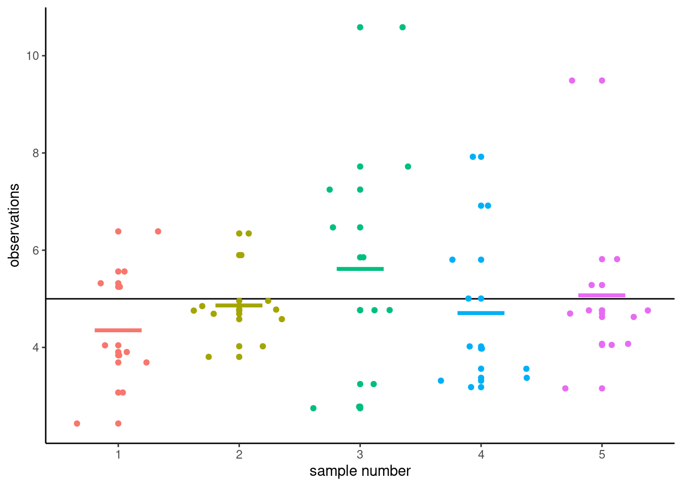
The astute eye might even notice that the sample means (thick horizontal segments) are less dispersed around the full black horizontal line representing the population average \(\mu\) than are the individual measurements. This is a fundamental principle of statistics: information accumulates as you get more data.

Values of the sample mean don’t tell the whole picture and studying differences in mean (between groups, or relative to a postulated reference value) is not enough to draw conclusions. In most settings, there is no guarantee that the sample mean will be equal to it’s true value because it changes from one sample to the next: the only guarantee we have is that it will be on average equal to the population average in repeated samples. Depending on the choice of measurement and variability in the population, there may be considerable differences from one observation to the next and this means the observed difference could be a fluke.

To get an idea of how certain something is, we have to consider the variability of an observation \(Y_i\). This variance of an observation drawn from the population is typically denoted \(\sigma^2\) and it’s square root, the standard deviation, by \(\sigma\).

The sample variance \(S_n\) is an estimator of the standard deviation \(\sigma\), where \[\begin{align*} S^2_n &= \frac{1}{n-1} \sum_{i=1}^n (Y_i-\overline{Y})^2 \end{align*}\] is the sum of squared difference between observations and the sample average, scaled by a factor proportional to the sample size.

The standard deviation of a statistic is termed standard error; it should not be confused with the standard deviation \(\sigma\) of the population from which the sample observations \(Y_1, \ldots, Y_n\) are drawn. Both standard deviation and standard error are expressed in the same units as the measurements, so are easier to interpret than variance. Since the standard error is a function of the sample size, it is however good practice to report the estimated standard deviation in reports.

Example 2.2 (Sample proportion and uniform draws) To illustrate the concept of sampling variability, we follow the lead of Matthew Crump and consider samples from a uniform distribution on \(\{1, 2, \ldots, 10\}\) each number in this interval is equally likely to be sampled.

Figure 2.5: Histograms for 10 random samples of size \(n=20\) from a discrete uniform distribution.

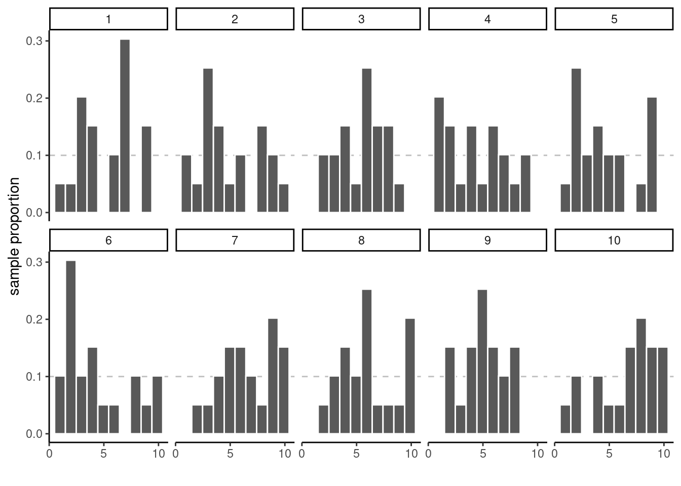
Even if they are drawn from the same population, the 10 samples in Figure 2.5 look quite different. The only thing at play here is the sample variability: since there are \(n=20\) observations in total, there should be on average 10% of the observations in each of the 10 bins, but some bins are empty and others have more counts than expected. This fluctuation is due to randomness, or chance.

How can we thus detect whether what we see is compatible with the model we think generated the data? The key is to collect more observations: the bar height is the sample proportion, an average of 0/1 values with ones indicating that the observation is in the bin and zero otherwise.

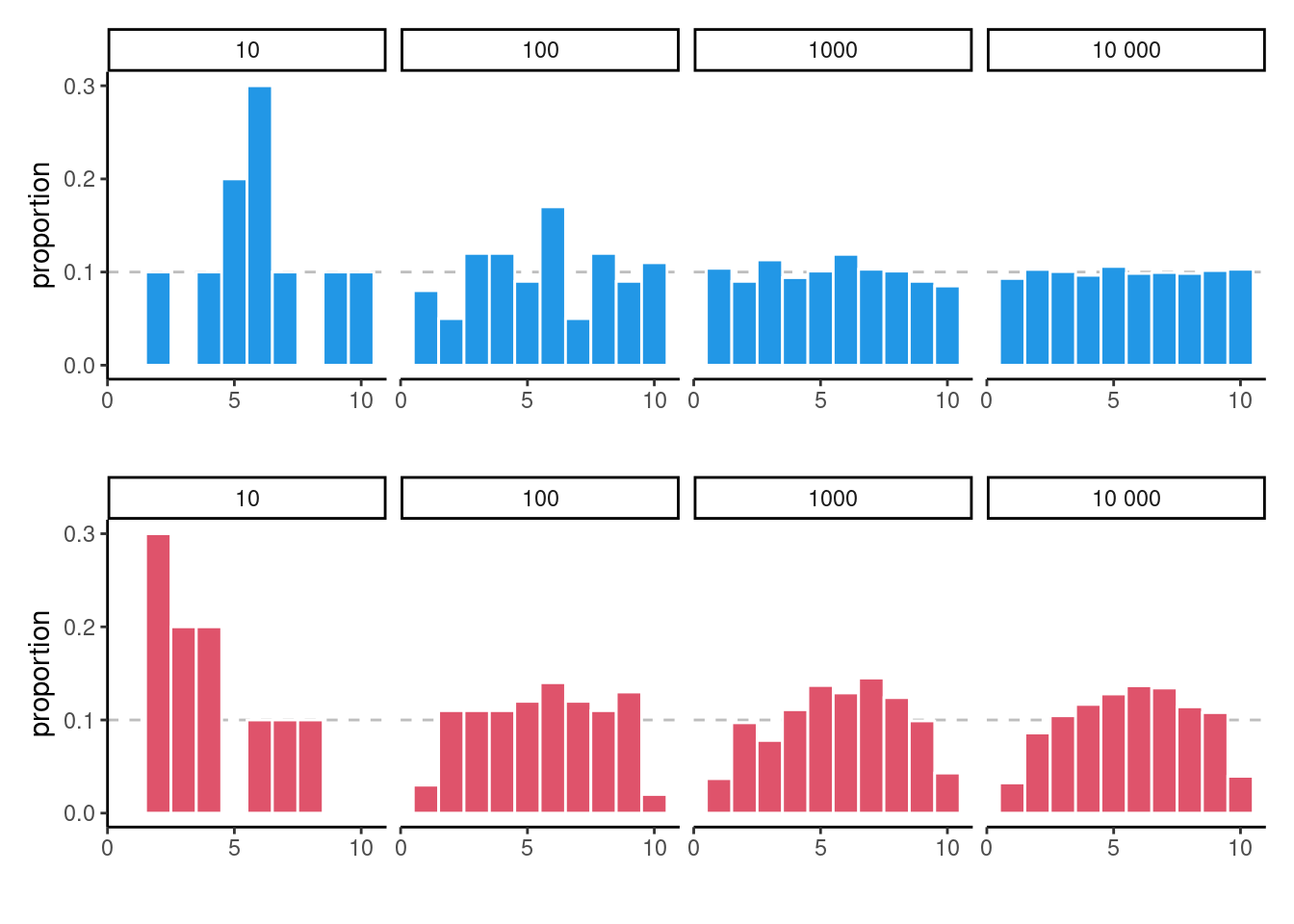
Consider now what happens as we increase the sample size: the top panel of Figure 2.6 shows uniform samples for increasing samples size. The histogram looks more and more like the true underlying distribution (flat, each bin with equal frequency) as the sample size increases. The sample distribution of points is nearly indistinguishable from the theoretical one (straight line) when \(n=10 000\).² The bottom panel, on the other hand, isn’t from a uniform distribution and larger samples come closer to the population distribution. We couldn’t have spotted this difference in the first two plots, since the sampling variability is too important; there, the lack of data in some bins could have been attributed to chance, as they are comparable with the graph for data that are truly uniform. This is in line with most practical applications, in which the limited sample size restricts our capacity to disentangle real differences from sampling variability. We must embrace this uncertainty: in the next section, we outline how hypothesis testing helps us disentangle the signal from the noise.

Figure 2.6: Histograms of data from a uniform distribution (top) and non-uniform (bottom) with increasing sample sizes of 10, 100, 1000 and 10 000 (from left to right).

2.3 Hypothesis testing

An hypothesis test is a binary decision rule (yes/no) used to evaluate the statistical evidence provided by a sample to make a decision regarding the underlying population. The main steps involved are:

• define the model parameters
• formulate the alternative and null hypothesis
• choose and calculate the test statistic
• obtain the null distribution describing the behaviour of the test statistic under \(\mathscr{H}_0\)
• calculate the p-value
• conclude (reject or fail to reject \(\mathscr{H}_0\)) in the context of the problem.

A good analogy for hypothesis tests is a trial for murder on which you are appointed juror.

• The judge lets you choose between two mutually exclusive outcome, guilty or not guilty, based on the evidence presented in court.
• The presumption of innocence applies and evidences are judged under this optic: are evidence remotely plausible if the person was innocent? The burden of the proof lies with the prosecution to avoid as much as possible judicial errors. The null hypothesis \(\mathscr{H}_0\) is not guilty, whereas the alternative \(\mathscr{H}_a\) is guilty. If there is a reasonable doubt, the verdict of the trial will be not guilty.
• The test statistic (and the choice of test) represents the summary of the proof. The more overwhelming the evidence, the higher the chance the accused will be declared guilty. The prosecutor chooses the proof so as to best outline this: the choice of evidence (statistic) ultimately will maximize the evidence, which parallels the power of the test.
• The null distribution is the benchmark against which to judge the evidence (jurisprudence). Given the proof, what are the odds assuming the person is innocent? Since this is possibly different for every test, it is common to report instead a p-value, which gives the level of evidence on a uniform scale which is most easily interpreted.
• The final step is the verdict, a binary decision with outcomes: guilty or not guilty. For an hypothesis test performed at level \(\alpha\), one would reject (guilty) if the p-value is less than \(\alpha\). Even if we declare the person not guilty, this doesn’t mean the defendant is innocent and vice-versa.

2.3.1 Hypothesis

In statistical tests we have two hypotheses: the null hypothesis (\(\mathscr{H}_0\)) and the alternative hypothesis (\(\mathscr{H}_a\)). Usually, the null hypothesis (the ‘status quo’) is a single numerical value. The alternative is what we’re really interested in testing. In Figure 2.4, we could consider whether all five groups have the same mean \(\mathscr{H}_0: \mu_1 = \mu_2 = \cdots = \mu_5\) against the alternative that at least two of them are different. These two outcomes are mutually exclusive and cover all possible scenarios. A statistical hypothesis test allows us to decide whether or not our data provides enough evidence to reject \(\mathscr{H}_0\) in favor of \(\mathscr{H}_a\), subject to some pre-specified risk of error: while we know that the differences are just due to sampling variability in Figure 2.4 because the data is simulated, in practice we need to assess the evidence using a numerical summary.

Example 2.3 (A/B testing (continued)) We follow-up with our A/B test experiment. Given \(\mu_1\) the population average click conversation rate for the current webpage and \(\mu_2\), that of the redesign, we are interested in the one-sided hypothesis that \(\mathscr{H}_0: \mu_2 \leq \mu_1\) against the alternative (that we are trying to prove) \(\mathscr{H}_a: \mu_2 > \mu_1\). In choosing as null hypothesis that the new design is no better or worst, we are putting all our weight to make sure the changes carry forward if there is overwhelming evidence that the new design is better and allow us to generate more revenues, given the costs associated to changes to the interface and the resulting disruption.

One-sided hypothesis are directional: we care only about a specific direction, and so here \(\mathscr{H}_a: \mu_2 > \mu_1\). Indeed, if the experiment suggests that the conversion rate is worst with the new webpage design, we won’t go forward.

Since neither of these population averages \(\mu_1\) and \(\mu_2\) are known to us, we can work instead with \(\mathscr{H}_0: \mu_2-\mu_1 \geq 0\). We can use as estimator for the difference \(\mu_2-\mu_1\) the difference in sample average in each subgroup.

The null hypothesis here is an interval, but it suffices the consider the most beneficial scenario, which is \(\mu_2-\mu_1=0\). Indeed, if we can disprove that there is no difference and see an increase of the click rate with the updated version, all more extreme cases are automatically discarded in favour of the alternative that the new design is better.

One-sided tests for which the evidence runs contrary to the hypothesis (say the mean conversion rate is higher for the current design than for the new one) lead to p-values of 1, since there is no proof against the null hypothesis that the old design (the status quo) is better.

The previous example illustrates the fact that, when writing down null and alternative hypotheses, what we are trying to prove is typically the alternative.

In pairwise comparisons or contrasts, we can assign a directionality. The benefit is that, if we are sure of the direction of the postulated effect, we only consider as extreme scenarios that run in the direction we postulated³ However, if the empirical evidence runs contrary to our guess, then there is no support for the hypothesis.

In more general statistical models, it helps to view the null hypothesis as a simplification of a more complex model: the latter will fit the data better because it is more flexible, but we would fail to reject the null unless this improvement is drastic. For example, in an analysis of variance model, we compare different mean in each of \(K\) groups against a single common average.

2.3.2 Test statistic

A test statistic \(T\) is a function of the data which takes the data as input and outputs a summary of the information contained in the sample for a characteristic of interest, say the population mean. In order to assess whether the numerical value for \(T\) is unusual, we need to know what are the potential values taken by \(T\) and their relative probability if \(\mathscr{H}_0\) is true. We need to know what values we should expect if, e.g., there was no difference in the averages of the different groups: this requires a benchmark.

Many statistics we will consider are of the form⁴ \[\begin{align*} T = \frac{\text{estimated effect}- \text{postulated effect}}{\text{estimated effect variability}} = \frac{\widehat{\theta} - \theta_0}{\mathrm{se}(\widehat{\theta})} \end{align*}\] where \(\widehat{\theta}\) is an estimator of \(\theta\), \(\theta_0\) is the postulated value of the parameter and \(\mathrm{se}(\widehat{\theta})\) is the standard error of the test statistic \(\widehat{\theta}\). This quantity is designed so that, if our postulated value \(\theta_0\) is correct, \(T\) has approximately mean zero and variance one. This standardization makes comparison easier; in fact, the form of the test statistic is chosen so that it doesn’t depend on the measurement units.

For example, if we are interested in mean differences between treatment group and control group, denoted \(\mu_T\) and \(\mu_C\), then \(\theta = \mu_T-\mu_C\) and \(\mathscr{H}_0: \mu_T = \mu_C\) corresponds to \(\mathscr{H}_0: \theta = 0\) for no difference. The two-sample \(t\)-test would have numerator \(\widehat{\theta} = \overline{Y}_T - \overline{Y}_C\), where \(\overline{Y}_T\) is the sample average in treatment group and \(\overline{Y}_C\) that of the control group. The postulated value for the mean difference is zero.

The numerator would thus consist of the difference in sample means and the denominator the standard error of that quantity, calculated using a software.⁵

2.3.3 Null distribution and p-value

The p-value allows us to decide whether the observed value of the test statistic \(T\) is plausible under \(\mathscr{H}_0\). Specifically, the p-value is the probability that the test statistic is equal or more extreme to the estimate computed from the data, assuming \(\mathscr{H}_0\) is true. Suppose that based on a random sample \(Y_1, \ldots, Y_n\) we obtain a statistic whose value \(T=t\). For a two-sided test \(\mathscr{H}_0:\theta=\theta_0\) vs. \(\mathscr{H}_a:\theta \neq \theta_0\), the p-value is \(\mathsf{Pr}_0(|T| \geq |t|)\).⁶

How do we determine the null distribution given that the true data generating mechanism is unknown to us? We ask a statistician! In simple cases, it might be possible to enumerate all possible outcomes and thus quantity the degree of outlyingness of our observed statistic. In more general settings, we can resort to simulations or to probability theory: the central limit theorem says that the sample mean behaves like a normal random variable with mean \(\mu\) and standard deviation \(\sigma/\sqrt{n}\) for \(n\) large enough. The central limit theorem has broader applications since most statistics can be viewed as some form of average or transformation thereof, a fact used to derive benchmarks for most commonly used tests. Most software use these approximations as proxy by default: the normal, Student’s \(t\), \(\chi^2\) and \(F\) distributions are the reference distributions that arise the most often.

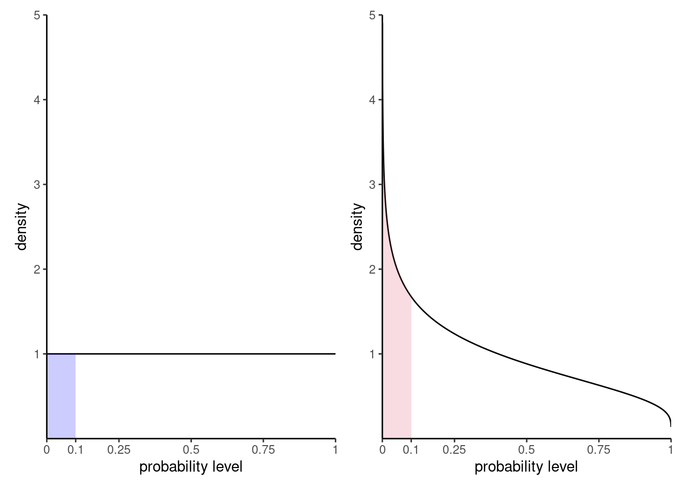
Figure 2.7 shows the distribution of \(p\)-values for two scenarios: one in which there are no differences and the null is true, the other under an alternative. The probability of rejection is obtained by calculating the area under the density curve between zero and \(\alpha=0.1\), here 0.1 on the left. Under the null, the model is calibrated and the distribution of p-values is uniform (i.e., a flat rectangle of height 1), meaning all values in the unit interval are equally likely. Under the alternative (right), small p-values are more likely to be observed.

Figure 2.7: Density of p-values under the null hypothesis (left) and under an alternative with a signal-to-noise ratio of 0.5 (right).

There are generally three ways of obtaining null distributions for assessing the degree of evidence against the null hypothesis

• exact calculations
• large sample theory (aka ‘asymptotics’ in statistical lingo)
• simulation

While desirable, the first method is only applicable in simple cases (such as counting the probability of getting two six if you throw two fair die). The second method is most commonly used due to its generality and ease of use (particularly in older times where computing power was scarce), but fares poorly with small sample sizes (where ‘too small’ is context and test-dependent). The last approach can be used to approximate the null distribution in many scenarios, but adds a layer of randomness and the extra computations costs sometimes are not worth it.

2.4 Confidence intervals

A confidence interval is an alternative way to present the conclusions of an hypothesis test performed at significance level \(\alpha\) by giving a range of all values for which the null isn’t rejected at the chosen level. It is often combined with a point estimator \(\hat{\theta}\) to give an indication of the variability of the estimation procedure. Wald-based \((1-\alpha)\) confidence intervals for a scalar parameter \(\theta\) are of the form \[\begin{align*} \widehat{\theta} + \text{critical value} \; \mathrm{se}(\widehat{\theta}) \end{align*}\] based on the Wald statistic \(W\), \[\begin{align*} W =\frac{\widehat{\theta}-\theta}{\mathrm{se}(\widehat{\theta})}, \end{align*}\] and where \(\theta\) represents the postulated value for the fixed, but unknown value of the parameter. The critical values are quantile of the null distribution and are chosen so that the probability of being more extreme is \(\alpha\).

The bounds of the confidence intervals are random variables, since both estimators of the parameter and its standard error, \(\widehat{\theta}\) and \(\mathrm{se}(\widehat{\theta})\), are random: their values will vary from one sample to the next.

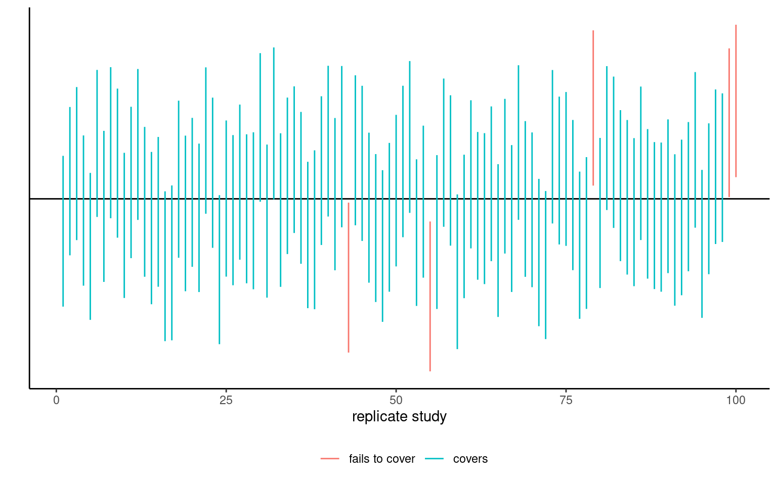
For generic random samples, there is a \(1-\alpha\) probability that \(\theta\) is contained in the random confidence interval computed. Once we obtain a sample and calculate the confidence interval, there is no more notion of probability: the true value of the parameter \(\theta\) is either inside the confidence interval or not. We can interpret confidence interval’s as follows: if we were to repeat the experiment multiple times, and calculate a \(1-\alpha\) confidence interval each time, then roughly \(1-\alpha\) of the calculated confidence intervals would contain the true value of \(\theta\) in repeated samples (in the same way, if you flip a coin, there is roughly a 50-50 chance of getting heads or tails, but any outcome will be either). Our confidence is in the procedure we use to calculate confidence intervals and not in the actual values we obtain from a sample.

95% confidence intervals for the mean of a standard normal population for 100 random samples. On average, 5% of these intervals fail to include the true mean value of zero (in red).

If we are only interested in the binary decision rule reject/fail to reject \(\mathscr{H}_0\), the confidence interval is equivalent to a p-value since it leads to the same conclusion. Whereas the \(1-\alpha\) confidence interval gives the set of all values for which the test statistic doesn’t provide enough evidence to reject \(\mathscr{H}_0\) at level \(\alpha\), the p-value gives the probability under the null of obtaining a result more extreme than the postulated value and so is more precise for this particular value. If the p-value is smaller than \(\alpha\), our null value \(\theta\) will be outside of the confidence interval and vice-versa.

2.4.1 Conclusion

The p-value allows us to make a decision about the null hypothesis. If \(\mathscr{H}_0\) is true, the p-value follows a uniform distribution, as shown in Figure 2.7. Thus, if the p-value is small, this means observing an outcome more extreme than \(T=t\) is unlikely, and so we’re inclined to think that \(\mathscr{H}_0\) is not true. There’s always some underlying risk that we’re making a mistake when we make a decision. In statistic, there are two type of errors:

• type I error: we reject the null hypothesis \(\mathscr{H}_0\) when the null is true,
• type II error: we fail to reject the null hypothesis \(\mathscr{H}_0\) when the alternative is true.

The two hypothesis are not judged equally: we seek to avoid error of type I (judicial errors, corresponding to condamning an innocent). To prevent this, we fix a the level of the test, \(\alpha\), which captures our tolerance to the risk of commiting a type I error: the higher the level of the test \(\alpha\), the more often we will reject the null hypothesis when the latter is true. The value of \(\alpha \in (0, 1)\) is the probability of rejecting \(\mathscr{H}_0\) when \(\mathscr{H}_0\) is in fact true, \[\begin{align*} \alpha = \mathsf{Pr}_0\left(\text{ reject } \mathscr{H}_0\right). \end{align*}\] The level \(\alpha\) is fixed beforehand, typically \(1\)%, \(5\)% or \(10\)%. Keep in mind that the probability of type I error is \(\alpha\) only if the null model for \(\mathscr{H}_0\) is correct (sic) and correspond to the data generating mechanism.

The focus on type I error is best understood by thinking about costs of moving away from the status quo: a new website design or branding will be costly to implement, so you want to make sure there are enough evidence that the proposal is the better alternative and will lead to increased traffic or revenues.

Decision \ true model	\(\mathscr{H}_0\)	\(\mathscr{H}_a\)
fail to reject \(\mathscr{H}_0\)	\(\checkmark\)	type II error
reject \(\mathscr{H}_0\)	type I error	\(\checkmark\)

To make a decision, we compare our p-value \(P\) with the level of the test \(\alpha\):

• if \(P < \alpha\), we reject \(\mathscr{H}_0\);
• if \(P \geq \alpha\), we fail to reject \(\mathscr{H}_0\).

Do not mix up level of the test (a probability fixed beforehand by the researcher) and the p-value. If you do a test at level 5%, the probability of type I error (condemning an innocent by mistake) is by definition \(\alpha\) and does not depend on the p-value. The latter is a conditional probability of observing a more extreme statistic given the null distribution \(\mathscr{H}_0\) is true.

Pitfall

The American Statistical Association (ASA) published a list of principles guiding (mis)interpretation of p-values, some of which are reproduced below:

2. P-values do not measure the probability that the studied hypothesis is true.

3. Scientific conclusions and business or policy decisions should not be based only on whether a p-value passes a specific threshold.

4. P-values and related analyses should not be reported selectively.

5. p-value, or statistical significance, does not measure the size of an effect or the importance of a result.

2.4.2 Examples

Example 2.4 (Gender inequality and permutation tests) We consider data from Rosen and Jerdee (1974), who look at sex role stereotypes and their impacts on promotion and opportunities for women candidates. The experiment took place in 1972 and the experimental units, which consisted of 95 male bank supervisors, were submitted to various memorandums and asked to provide ratings or decisions based on the information provided.

We are interested in Experiment 1 related to promotion of employees: managers were requested to decide on whether or not to promote an employee to become branch manager based on recommendations and ratings on potential for customer and employee relations.

The authors intervention focused on the description of the nature (complexity) of the manager’s job (either simple or complex) and the sex of the candidate (male or female): all files were otherwise similar.

We consider for simplicity only sex as a factor and aggregate over job for the \(n=93\) replies. Table 2.1 shows the counts for each possibility.

Table 2.1: Promotion recommandation to branch manager based on sex of the applicant.

	male	female
promote	32	19
hold file	12	30

The null hypothesis of interest here that sex has no impact, so the probability of promotion is the same for men and women. Let \(p_{\text{m}}\) and \(p_{\text{w}}\) denote these respective probabilities; we can thus write mathematically the null hypothesis as \(\mathscr{H}_0: p_{\text{m}} = p_{\text{w}}\) against the alternative \(\mathscr{H}_a: p_{\text{m}} \neq p_{\text{w}}\).

The test statistic typically employed for contingency tables is a chi-square test⁷, which compares the overall proportions of promoted to that in for each subgroup. The sample proportion for male is 32/42 = ~76%, compared to 19/49 or ~49% for female. While it seems that this difference of 16% is large, it could be spurious: the standard error for the sample proportions is roughly 3.2% for male and 3.4% for female.

If there was no discrimination based on sex, we would expect the proportion of people promoted to be the same overall; this is 51/93 =0.55 for the pooled sample. We could simply do a test for the mean difference, but rely instead on the Pearson contingency \(X^2_p\) (aka chi-square) test, which compares the expected counts (based on equal promotion rates) to the observed counts, suitably standardized. If the discrepancy is large between expected and observed, than this casts doubt on the validity of the null hypothesis.

If the counts of each cell are large, the null distribution of the chi-square test is well approximated by a \(\chi^2\) distribution. The output of the test includes the value of the statistic, \(10.79\), the degrees of freedom of the \(\chi^2\) approximation and the p-value, which gives the probability that a random draw from a \(\chi^2_1\) distribution is larger than the observed test statistic assuming the null hypothesis is true. The p-value is very small, \(0.001\), which means such a result is quite unlikely to happen by chance if there was no sex-discrimination.

Another alternative to obtain a benchmark to assess the outlyingness of the observed odds ratio is to use simulations: permutation tests are well illustrated by Jared Wilber. Consider a database containing the raw data with 93 rows, one for each manager, with for each an indicator of action and the sex of the hypothetical employee presented in the task.

Table 2.2: First five rows of the database in long format for experiment 1 of Rosen and Jerdee.

action	sex
promote	male
hold file	female
promote	male
hold file	female
hold file	male

Under the null hypothesis, sex has no incidence on the action of the manager. This means we could get an idea of the “what-if” world by shuffling the sex labels repeatedly. Thus, we could obtain a benchmark by repeating the following steps multiple times:

1. permute the labels for sex,
2. recreate a contingency table by aggregating counts,
3. calculate a test statistic for the simulated table.

As test statistic, we use odds ratio: the odds of an event is the ratio of the number of success over failure: in our example, this would be the number of promoted over held files. The odds of promotion for male is \(32/12\), whereas that of female is \(19/30\). The odds ratio for male versus female is thus \(\mathsf{OR}=(32/12) / (19/30)= 4.21\). Under the null hypothesis, \(\mathscr{H}_0: \mathsf{OR}= 1\) (same probability of being promoted) (why?)

Figure 2.8: Histogram of the simulated null distribution of the odds ratio statistic obtained using a permutation test; the vertical red line indicates the sample odds ratio.

The histogram in Figure 2.8 shows the distribution of the odds ratio based on 10 000 permutations. Reassuringly, we again get roughly the same approximate p-value, here 0.002.⁸

The article concluded (in light of the above and further experiments)

Results confirmed the hypothesis that male administrators tend to discriminate against female employees in personnel decisions involving promotion, development, and supervision.

Recap

• Model parameters: probability of promotion for men and women, respectively \(p_{\text{m}}\) and \(p_{\text{w}}\).
• Hypotheses: no discrimination based on gender, meaning equal probability of promotion (null hypothesis \(\mathscr{H}_0: p_{\text{m}}=p_{\text{w}}\), versus alternative hypothesis \(\mathscr{H}_a: p_{\text{m}}\neq p_{\text{w}}\)).
• Test statistic: (1) chi-square test for contingency tables and (2) odds ratio.
• \(p\)-value: (1) \(.0010\) and (2) \(.0024\) based on permutation test.
• Conclusion: reject null hypothesis, as there is evidence of a gender-discrimination with different probability of promotion for men and women.

Following the APA guidelines, the \(\chi^2\) statistic would be reported as \(\chi^2(1, n = 93) = 10.79\), \(p = .001\) along with counts and sample proportions.

Pitfall

In the first experiment, managers were also asked to rank applications on their potential for both employee and customer relations using a Likert scale of six items ranging from (1) extremely unfavorable to (6) extremely favorable. However, only the averages are reported in Table 1 along with (Rosen and Jerdee 1974)

Mean rating for the male candidate was 4.73 compared to a mean rating of 4.25 for the female candidate (\(F=4.76\), \(\text{df} = 1/80\), \(p < .05\))

The degrees of freedom (80) are much too few compared to the number of observations, implying non-response that isn’t discussed.

Partial or selective reporting of statistical procedures hinders reproducibility. In general, the presentation should explicitly state the name of the test statistic employed, the sample size, mean and variance estimates, the null distribution used to assess significance and its parameters, if any. Without these, we are left to speculate.

Example 2.5 (“The Surprise of Reaching Out”) Liu et al. (2023) studies social interactions and the impact of surprise on people reaching out if this contact is unexpected. Experiment 1 focuses on questionnaires where the experimental condition is the perceived appreciation of reaching out to someone (vs being reached to). The study used a questionnaire administered to 200 American adults recruited on the Prolific Academic platform. The response index consists of the average of four questions measured on a Likert scale ranging from 1 to 7, with higher values indicating higher appreciation.

We can begin by inspecting summary statistics for the sociodemographic variables (gender and age) to assess whether the sample is representative of the general population as a whole. The proportion of other (including non-binary people) is much higher than that of the general census, and the population skews quite young according to Table 2.3.

Table 2.3: Summary statistics of the age of participants, and counts per gender

gender	min	max	mean	n
male	18	78	32.03	105
female	19	68	36.50	92
other	24	30	27.67	3

Table 2.4: Mean ratings, standard deviation and number of participants per experimental condition.

role	mean	sd	n
initiator	5.50	1.28	103
responder	5.87	1.27	97

Since there are only two groups, initiator and responder, we are dealing with a pairwise comparison. The logical test one could use is a two sample t-test, or a variant thereof. Using Welch two sample \(t\)-test statistic, both group average and standard deviation are estimated using the data provided and the latter are used to build a statistic. This explains the non-integer degrees of freedom.

The software returns \(t(197.52) = -2.05\), \(p = .041\), which leads to the rejection of the null hypothesis of no difference in appreciation depending on the role of the individual (initiator or responder). The estimated mean difference is \(\Delta M = -0.37\), 95% CI \([-0.73, -0.01]\); since \(0\) is not included in the confidence interval, we also reject the null hypothesis at level 5%. The estimate suggests that initiators underestimate the appreciation of reaching out.⁹

Recap

• Model parameters: average expected appreciation score \(\mu_{\mathrm{i}}\) and \(\mu_{\mathrm{r}}\) of initiators and responder, respectively
• Hypothesis: expected appreciation score is the same for initiator and responders, \(\mathscr{H}_0: \mu_{\mathrm{i}}=\mu_{\mathrm{r}}\) against alternative \(\mathscr{H}_0: \mu_{\mathrm{i}} \neq \mu_{\mathrm{r}}\) that they are different.
• Test statistic: Welch two sample \(t\)-test
• \(p\)-value: 0.041
• Conclusion: reject the null hypothesis, average appreciation score differs depending on the role

Example 2.6 (Virtual communication curbs creative idea generation) A Nature study performed an experiment to see how virtual communications teamwork by comparing the output both in terms of ideas generated during a brainstorming session by pairs and of the quality of ideas, as measured by external referees. The sample consisted of 301 pairs of participants who interacted via either videoconference or face-to-face.

The authors compared the number of creative ideas, a subset of the ideas generated with creativity score above average. The mean number of the number of creative ideas for face-to-face \(7.92\) ideas (sd \(3.40\)) relative to videoconferencing \(6.73\) ideas (sd \(3.27\)).

Brucks and Levav (2022) used a negative binomial regression model: in their model, the expected number creative ideas generated is \[\begin{align*} \mathsf{E}(\texttt{ncreative}) = \exp(\beta_0 + \beta_1 \texttt{video}) \end{align*}\] where \(\texttt{video}=0\) if the pair are in the same room and \(\texttt{video}=1\) if they interact instead via videoconferencing.

The mean number of ideas for videoconferencing is thus \(\exp(\beta_1)\) times that of the face-to-face: the estimate of the multiplicative factor is \(\exp(\beta_1)\) is \(0.85\) 95% CI \([0.77, 0.94]\).

No difference between experimental conditions translates into the null hypothesis as \(\mathscr{H}_0: \beta_1=0\) vs \(\mathscr{H}_0: \beta_1 \neq 0\) or equivalently \(\mathscr{H}_0: \exp(\beta_1)=1\). The likelihood ratio test comparing the regression model with and without \(\texttt{video}\) the statistic is \(R=9.89\) (\(p\)-value based on \(\chi^2_1\) of \(.002\)). We conclude the average number of ideas is different, with summary statistics suggesting that virtual pairs generate fewer ideas.

If we had resorted to a two sample \(t\)-test, we would have found a mean difference in number of creative idea of \(\Delta M = 1.19\), 95% CI \([0.43, 1.95]\), \(t(299) = 3.09\), \(p = .002\).

Both tests come with slightly different sets of assumptions, but yield similar conclusions: there is evidence of a smaller number of creative ideas when people interact via videoconferencing.

2.5 Conclusion

This chapter has focused on presenting the tools of the trade and some examples outlining the key ingredients that are common to any statistical procedure and the reporting of the latter. The reader is not expected to know which test statistic to adopt, but rather should understand at this stage how our ability to do (scientific) discoveries depends on a number of factors.

Richard McElreath in the first chapter of his book (McElreath 2020) draws a parallel between statistical tests and golems (i.e., robots): neither

discern when the context is inapropriate for its answers. It just knows its own procedure […] It just does as it’s told.

The responsibility therefore lies with the user to correctly use statistical procedures and be aware of their limitations. A p-value does not indicate whether the hypothesis is reasonable, whether the design is proper, whether the choice of measurement is adequate, etc.

Your turn

Pick a journal paper (e.g., one of the dataset documented in the course webpage) and a particular study.

Look up for the ingredients of the testing procedure (parameters, hypotheses, test statistic name and value, summary statistics, p-value, conclusion).

You may encounter other measures, such as effect size, that will be discussed later.

Brucks, Melanie S., and Jonathan Levav. 2022. “Virtual Communication Curbs Creative Idea Generation.” Nature 605 (7908): 108–12. https://doi.org/10.1038/s41586-022-04643-y.

Liu, Peggy J., SoYon Rim, Lauren Min, and Kate E. Min. 2023. “The Surprise of Reaching Out: Appreciated More Than We Think.” Journal of Personality and Social Psychology 124 (4): 754–71. https://doi.org/10.1037/pspi0000402.

McElreath, R. 2020. Statistical Rethinking: A Bayesian Course with Examples in r and Stan. 2nd ed. CRC Press. https://www.routledge.com/Statistical-Rethinking-A-Bayesian-Course-with-Examples-in-R-and-STAN/McElreath/p/book/9780367139919.

Rosen, B., and T. H. Jerdee. 1974. “Influence of Sex Role Stereotypes on Personnel Decisions.” Journal of Applied Psychology 59: 9–14.

---

1. We could look at the ratio \(\mu_T/\mu_C\) instead.

2. The formula shows that the standard error decreases by a tenfold every time the sample size increases by a factor 100.

3. This implies that the level \(\alpha\) is all on one side, rather than split equally between both tails of the distribution. In practice, this translates into increased power of detection provided the effect is in the postulated direction.

4. This class of statistic, which includes \(t\)-tests, are called Wald statistics.

5. Assuming equal variance, the denominator is estimated using the pooled variance estimator.

6. If the distribution of \(T\) is symmetric around zero, the p-value reduces to \(p = 2 \times \mathsf{Pr}_0(T \geq |t|).\)

7. If you have taken advanced modelling courses, this is a score test obtained by fitting a Poisson regression with sex and action as covariates; the null hypothesis corresponding to lack of interaction term between the two.

8. The p-value obtained for the permutation test would change from one run to the next since it’s input is random. However, the precision of the proportion statistic is sufficient for decision making purposes.

9. Assuming that the variance of each subgroup were equal, we could have used a two-sample \(t\)-test instead. The difference in the conclusion is immaterial, with a nearly equal p-value.