8.1 Bias and variance tradeoff

As we increase the penalty $\lambda$, the values of the ridge coefficients are shrunk towards zero. The case $\lambda \to \infty$ gives $\hat{\boldsymbol{\beta}}_{\mathrm{ridge}}=\boldsymbol{0}_p$, whereas we retrieve the OLS estimator $\hat{\boldsymbol{\beta}}$ when $\lambda=0$.

The mean squared error of the ridge estimator is $$\begin{align*} \mathrm{MSE}(\hat{\boldsymbol{\beta}}_{\mathrm{ridge}}^{\lambda}) &= \sigma^2 \mathrm{tr}\left\{(\mathbf{Z}^\top\mathbf{Z} + \lambda \mathbf{I}_p)^{-1}\mathbf{Z}^\top\mathbf{Z}(\mathbf{Z}^\top\mathbf{Z} + \lambda \mathbf{I}_p)^{-1}\right\} \\&\quad + \boldsymbol{\gamma}^\top \left\{ \mathbf{Z}^\top\mathbf{Z}(\mathbf{Z}^\top\mathbf{Z} + \lambda \mathbf{I}_p)^{-1} + \mathbf{I}_p \right\} \left\{ (\mathbf{Z}^\top\mathbf{Z} + \lambda \mathbf{I}_p)^{-1}\mathbf{Z}^\top\mathbf{Z} + \mathbf{I}_p \right\}\boldsymbol{\gamma} \end{align*}$$

If we knew the true data generating mechanism (i.e. the $\boldsymbol{\gamma}$ vector and $\sigma^2$), we could compute exactly the mean squared error (MSE) of the model and find the optimal bias-variance tradeoff that minimizes MSE. This is illustrated below in an artificial example. As $\lambda \to \infty$, the bias grows and dominates MSE.

# Function to compute MSE of ridge estimator
mse_ridge <- function(gamma, lambda, Z, sigmasq = 1){
  ZtZ <- crossprod(Z)
  p <- ncol(Z)
  W <- solve(ZtZ + lambda*diag(p))
  bias <- c((W %*% ZtZ - diag(p)) %*% gamma)
  varia <- sigmasq * diag( crossprod(Z %*% W))
  list(bias = bias, variance = varia, mse = sum(bias^2 + varia))
}
set.seed(9876)
# Create fake data
Z <- matrix(rnorm(n = 20L*50L, mean = 0, sd = 1), ncol = 20L)
# Center and renormalize Z
Z <- apply(Z, 2, scale)
# Create coefficient vector
gamma <- c(rep(0, 10L), runif(10L))

# Create sequence of lambda and matrix to store results
nlam <- 401L
lambda_seq <- seq(0, 100, length = nlam)
mse <- matrix(0, nrow = nlam, ncol = 3)
gammahat <- matrix(0, nrow = nlam, ncol = ncol(Z))
for(i in 1:nlam){
  # evaluate bias + variance for each lambda
  mse_i <- mse_ridge(gamma = gamma, lambda = lambda_seq[i], Z = Z)
  gammahat[i,] <- gamma + mse_i$bias
  mse[i,1] <-  sum(mse_i$bias^2)
  mse[i,2] <-  sum(mse_i$variance)
  mse[i,3] <- mse_i$mse
}
# Plot the results as a function of lambda
matplot(lambda_seq, mse, type = "l", lty = 1, 
        bty = "l", xlab = expression(lambda), col = 3:1, 
        ylab = "Mean squared error decomposition")
abline(h = mse[1,3], lty = 2)
legend(x = "topleft", legend = c("sq. bias", "variance", "mse"), 
       col = 3:1, lty = 1, bty = "n")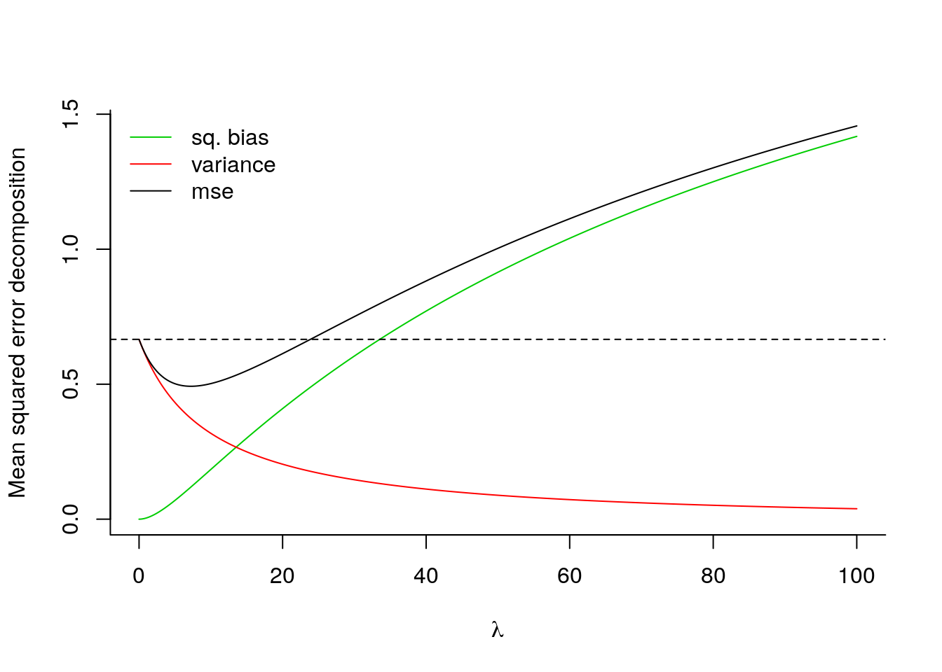

# Compute the value of lambda that minimizes MSE
lambdaopt <- optimize(f = function(x){
  mse_ridge(gamma = gamma, lambda = x, Z = Z)$mse
  }, interval = c(0, 30))$minimum
lambdaopt

## [1] 7.227898

We can also look at the path of coefficient values $\hat{\boldsymbol{\gamma}}_{\mathrm{ridge}}^{\lambda}$ as a function of $\lambda$:

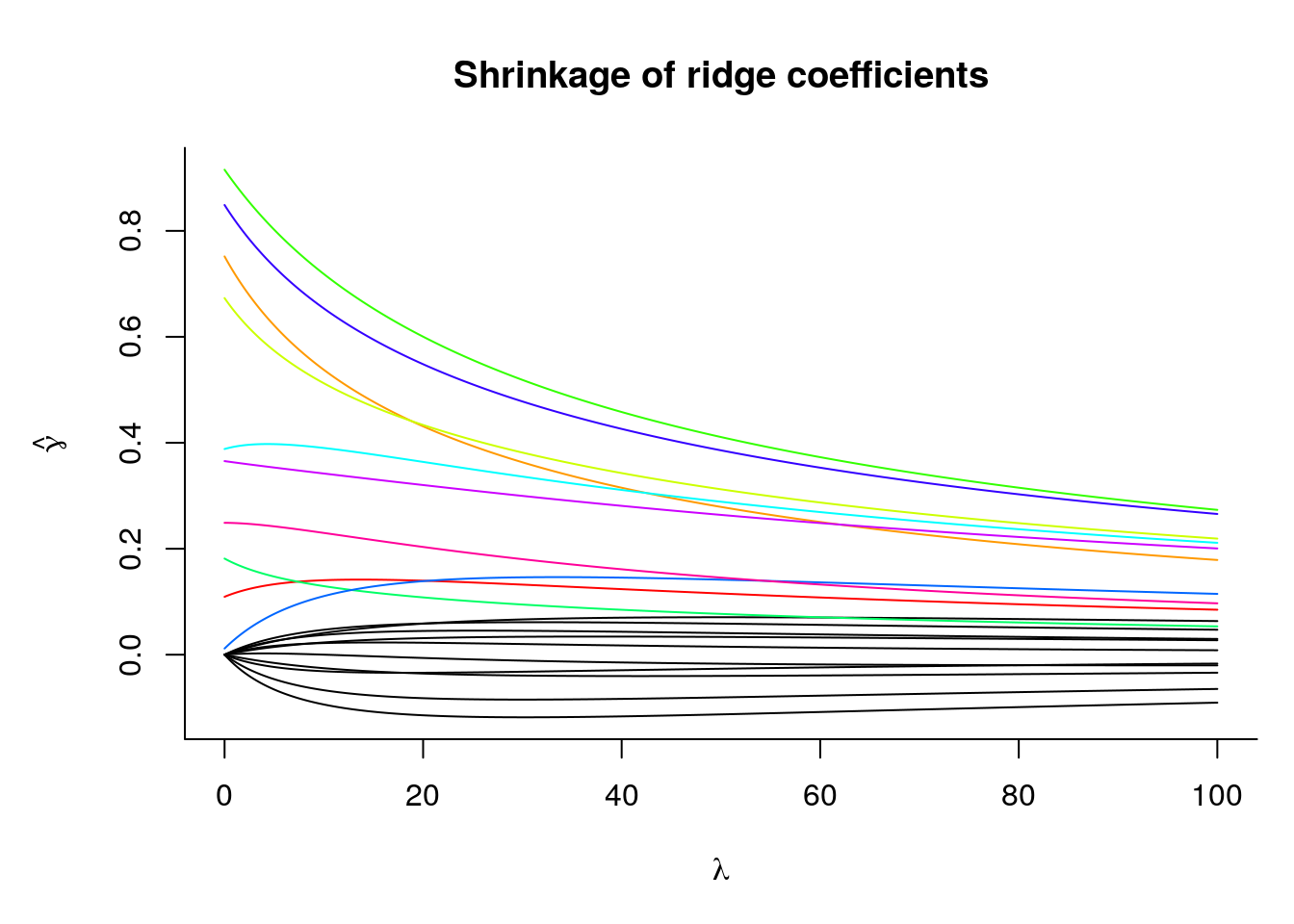
While the overall vector of coefficients are shrunk towards zero, the set of 10 first coefficients $\boldsymbol{\gamma}$, which are exactly zero, stabilize around another value. Note that if we increase the penalty, from $\lambda_1$ to $\lambda_2$ with $\lambda_1 < \lambda_2$, this does not necessarily imply that individual coefficient estimates decrease, i.e. $|\hat{\beta}_j (\lambda_1)| \nleq |\hat{\beta}_j(\lambda_2)|$ even if $\lambda_1 < \lambda_2$.

The coefficients $\hat{\boldsymbol{\gamma}}^\lambda$ can be computed using an augmented linear regression, with response $(\boldsymbol{y}, \mathbf{0}_p)$ and regressor $[\mathbf{Z}^\top,\; \lambda^{1/2} \mathbf{I}_p]$. Alternatively, $$\hat{\boldsymbol{\gamma}}^\lambda = (\mathbf{Z}^\top\mathbf{Z} + \lambda \mathbf{I}_p)^{-1}\mathbf{Z}^\top\boldsymbol{y}.$$

We can also use the singular value decomposition of $\mathbf{Z} = \mathbf{UDV}^\top$ to compute the coefficients $$\hat{\boldsymbol{\gamma}} = \sum_{j=1}^p \frac{d_j}{d_j^2+\lambda} \mathbf{u}_j^\top\boldsymbol{y} \mathbf{v}_j,$$ where $\mathbf{u}_j$ and $\mathbf{v}_j$ are the $j$th column of $\mathbf{U}$ and $\mathbf{V}$, respectively. This is most useful for cross-validation where we want to change the value of $\lambda$ repeatedly, as the SVD of $\mathbf{Z}$ won’t change.

# Create response vector from model
y <- Z %*% gamma + rnorm(nrow(Z))
# Compute ridge coefficients
ridge_lm_coef <- function(y, Z, lambda){
 Z <- scale(Z) 
 c(solve(crossprod(Z) + lambda*diag(ncol(Z))) %*% crossprod(Z, y - mean(y)))
}
lambda0 <- 2
#Compare coefficients obtained from fitting using augmented regression
augmy <- c(y - mean(y), rep(0, ncol(Z)))
augmZ <- rbind(Z, sqrt(lambda0)*diag(ncol(Z)))
augmlm <- lm(augmy ~ -1 + augmZ)
isTRUE(all.equal(as.vector(augmlm$coef),
      ridge_lm_coef(y = y, Z = Z, lambda = lambda0)))

## [1] TRUE