4.1 Confidence and prediction intervals

In the linear model with IID errors $\boldsymbol{\varepsilon}\sim \mathsf{IID}(0, \sigma^2)$, we have $\mathsf{Var}(\hat{\boldsymbol{\beta}}) = \sigma^2(\mathbf{X}^\top\mathbf{X})^{-1}$. The standard errors for $\hat{\boldsymbol{\beta}}$ are then simply the square root of the diagonal entries (which are the variance $\mathsf{Var}(\hat{\beta}_j)$ for $j=1, \ldots, p$. Confidence intervals for the coefficients are given by $\hat{\beta}_i \pm t_{n-p}({0.025})\mathsf{se}(\hat{\beta}_i)$.

We can also draw intervals around the regression line by considering combinations $\mathbf{x} = (1, \texttt{mpg})$ for different values of $\texttt{mpg}$ as illustrated below. The reasoning is similar, except that we now obtain the interval for a function of $\widehat{\boldsymbol{\beta}}$. For each new vector of regressors $\mathbf{x}^i \equiv \mathbf{c}$, we get new fitted values $\hat{y}^i= \mathbf{x}^i\widehat{\boldsymbol{\beta}}$ whose variance is, by the delta-method, given by $\mathsf{Var}(y^i)={\sigma^2}\mathbf{x}^{i\top}(\mathbf{X}^\top\mathbf{X})^{-1}\mathbf{x}^i$. We replace $\sigma^2$ by the usual estimator $s^2$ and thus the pointwise confidence interval is given by the usual Student-$t$ test statistics, with this time \[\hat{y}^i \pm t_{n-p}({0.025})\mathsf{se}(\hat{y}^i) = \mathbf{x}^i\widehat{\boldsymbol{\beta}} \pm t_{n-p}({0.025})\sqrt{s^2\mathbf{x}^{i\top}(\mathbf{X}^\top\mathbf{X})^{-1}\mathbf{x}^i}.\]

For the prediction interval, we consider instead \[ \mathbf{x}^i\widehat{\boldsymbol{\beta}} \pm t_{n-p}({0.025})\sqrt{s^2 \left[ \mathbf{I}_n + \mathbf{x}^{i\top}(\mathbf{X}^\top\mathbf{X})^{-1}\mathbf{x}^i\right]}.\] Provided the model is correct, new observations $y_{\mathrm{new}}$ should fall 19 times out of 20 within the reported prediction interval.

As we move away from the bulk of the data (average value of $\mathbf{x}$), the hyperbolic shape of the intervals becomes visible. Note here how the prediction interval is necessarily wider than the confidence interval (iterated variance formula).

# The function lm and its output
ols <- lm(mpg ~ wt, data = mtcars)
res <- resid(ols)
X <- cbind(1,  mtcars$wt)
n <- nrow(X)
s2 <- sum(res^2) / (length(res) - ncol(X))
std_err <- sqrt(diag(s2 * solve(crossprod(X))))
beta_hat <- coef(ols)
#Covariance matrix of (beta0, beta1)
Sigma <- vcov(summary(ols))
#check the calculation
isTRUE(all.equal(Sigma, s2 * solve(crossprod(X)), check.attributes = FALSE))

## [1] TRUE

#Standard error of estimates
std_err <- sqrt(diag(Sigma))
#Extract leverage values h_ii
leverage <- as.vector(hatvalues(ols))
# Compare with manual calculation from diagonal matrix
leverage_man <- rep(0, n)
XtXinv <- solve(crossprod(X))
for(i in 1:n){
  leverage_man[i] <- X[i,] %*% XtXinv %*% X[i,]
}
isTRUE(all.equal(leverage, leverage_man))

## [1] TRUE

# Plot data set
plot(mpg ~ wt, data = mtcars, 
     xlab = "weight (1000 lbs)", 
     ylab = "Fuel consumption (in miles/US gallon)", 
     main = "Fuel consumption of automobiles, 1974 Motor Trend", 
     bty = "l", pch = 20, ylim = c(0, 35), xlim = c(0, 6))
abline(beta_hat, col = 'red', lwd = 2)

#Confidence intervals
tqu = qt(0.975, df = nrow(X)- ncol(X))
conf_inter <- cbind(beta_hat - tqu * std_err, beta_hat + tqu * std_err)
#Compare with lm output
confint(ols)

##                 2.5 %    97.5 %
## (Intercept) 33.450500 41.119753
## wt          -6.486308 -4.202635

xstar <- seq(0, 6, by = 0.1)

#Confidence interval for prediction using lm output
ystar_confint <- predict(ols, newdata = data.frame(wt = xstar), interval = 'confidence')
lines(xstar, ystar_confint[ ,2], lty = 2, col = 'green')
lines(xstar, ystar_confint[ ,3], lty = 2, col = 'green')
#Prediction interval using lm output
ystar_predint <- predict(ols, newdata = data.frame(wt = xstar), interval = 'prediction')
lines(xstar, ystar_predint[ ,2], lty = 2, col = 'blue')
lines(xstar, ystar_predint[ ,3], lty = 2, col = 'blue')
legend(x = "topright", col = c("red", "green","blue"), 
       lty = c(1, 2, 2), bty = "n",
       legend = c("Prediction","Conf. inter.","Pred. inter."))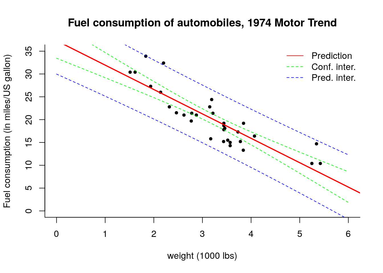

The function predict takes as imput a data.frame object containing the same column names as those of the fitted lm object. The names can be obtained from names(ols$model)[-1].

As usual, we can verify we get the same result if we computed the intervals manually.

#Manually (see class notes)
confint_xstar <- tqu * sqrt(s2 * apply(cbind(1, xstar), 1, function(cvec){t(cvec) %*% solve(crossprod(X)) %*% cvec}))
fitted_xstar <- cbind(1, xstar) %*% cbind(beta_hat)
lines(xstar,  fitted_xstar - confint_xstar, lty = 2, col = 'green')
lines(xstar,  fitted_xstar + confint_xstar, lty = 2, col = 'green')