8.2 Cross-validation
Denote the ridge estimator \(\hat{\boldsymbol{\beta}}^\lambda\) for a given penalty parameter \(\lambda\). The smoothing matrix, as given in the course notes, is \[\mathbf{S}_{\lambda} = \mathbf{Z}(\mathbf{Z}^\top\mathbf{Z} + \lambda \mathbf{I}_p)^{-1}\mathbf{Z}^\top;\] its trace is \(\mathrm{tr}({\mathbf{S}_{\lambda}}) = \sum_{j=1}^p d_j^2/(d_j^2+\lambda)\), where \(d_{j}\) is the \(j\)th singular value of \(\mathbf{Z}\). The smoothing matrix \(\mathbf{S}_{\lambda}\) is not a projection matrix; its eigenvalues lie in \((0,1)\).
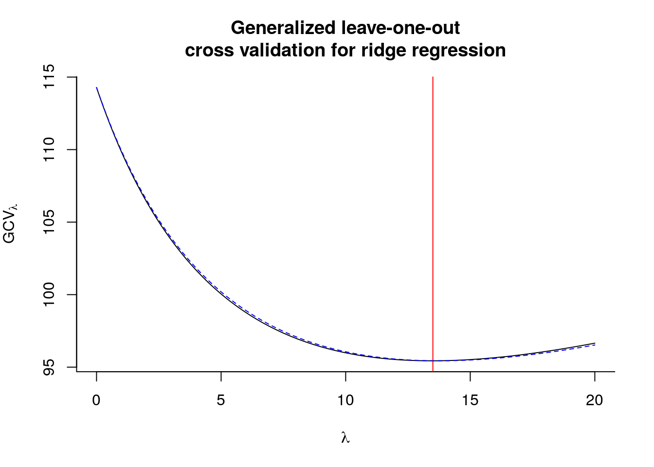
Similar calculations than those used to derive the leave-one-out cross validation residual errors of the PRESS statistic lead to the formula \[\mathrm{CV}_\lambda = \sum_{i=1}^n e_{-i}^2(\lambda) = \sum_{i=1}^n (y_i - \bar{y}- \mathbf{z}_i \hat{\boldsymbol{\gamma}}_{-i}^{\lambda})^2 = \sum_{i=1}^n \frac{(y_i - \bar{y} -\mathbf{z}_i\hat{\boldsymbol{\gamma}}^\lambda)^2}{1-{\mathbf{S}_{\lambda}}_{ii}},\] where \(\mathbf{z}_i\) is the \(i\)th row of \(\mathbf{Z}\). Rather than compute \(\mathbf{S}_{\lambda}\) and its diagonal elements, one can resort to the convenient generalized cross-validation approximation \[\mathrm{GCV}_\lambda = \sum_{i=1}^n \frac{(y_i - \bar{y} -\mathbf{z}_i\hat{\boldsymbol{\gamma}}^\lambda)^2}{1-\mathrm{tr}(\mathbf{S}_{\lambda})/n}\] and the latter is readily computed.
nlam <- 201L
lambda_seq <- seq(0, 20, length = nlam)
svdZ <- svd(Z)
n <- nrow(Z); p <- ncol(Z)
#Each column is u_j^Tyv_j
uyv <- sapply(1:p, function(j){t(svdZ$u[,j]) %*% y %*% svdZ$v[,j]})
gcv <- rep(0, nlam)
yc <- y - mean(y)
for(i in 1:nlam){
  # Compute GCV - trace of smoother + RSS
  traceS <- sum(svdZ$d^2/(svdZ$d^2+lambda_seq[i]))
  gcv[i] <- sum((yc - Z %*% colSums(c(svdZ$d/(svdZ$d^2 + lambda_seq[i]))  *
                                      t(uyv)))^2)/(1-traceS/n)^2
}
# Plot GCV curve against lambda
plot(lambda_seq, gcv, type = "l", bty = "l",
     main = "Generalized leave-one-out\ncross validation for ridge regression",
     ylab = expression(GCV[lambda]), xlab = expression(lambda))
abline(v = lambda_seq[which.min(gcv)], col = 2)
lambda_seq[which.min(gcv)]
## [1] 13.5# Compare results with MASS
library(MASS)
fit_ridge <- lm.ridge(y ~ Z, lambda = lambda_seq)
# GCV returned by lm.ridge is divided by n^2
lines(lambda_seq, fit_ridge$GCV*n^2, lty = 2, col = "blue")
## modified HKB estimator is 8.577316
## modified L-W estimator is 7.881568
## smallest value of GCV  at 13.7
Note that in this case, the optimal value of \(\lambda\) found is higher than the theoretical optimum. In practice, we may prefer \(K\)-fold cross-validation to leave-one-out cross validation.