9 Splines
The following code provides functions to compute manually a cubic spline and returns the penalty function. In R, one would rather use functions that compute efficiently the generalized cross-validation criterion and return the best smoothing or regression spline.
The package splines contains bs for cubic regression splines and ns for natural regression splines. Smoothing splines can be obtained by a call to smooth.spline.
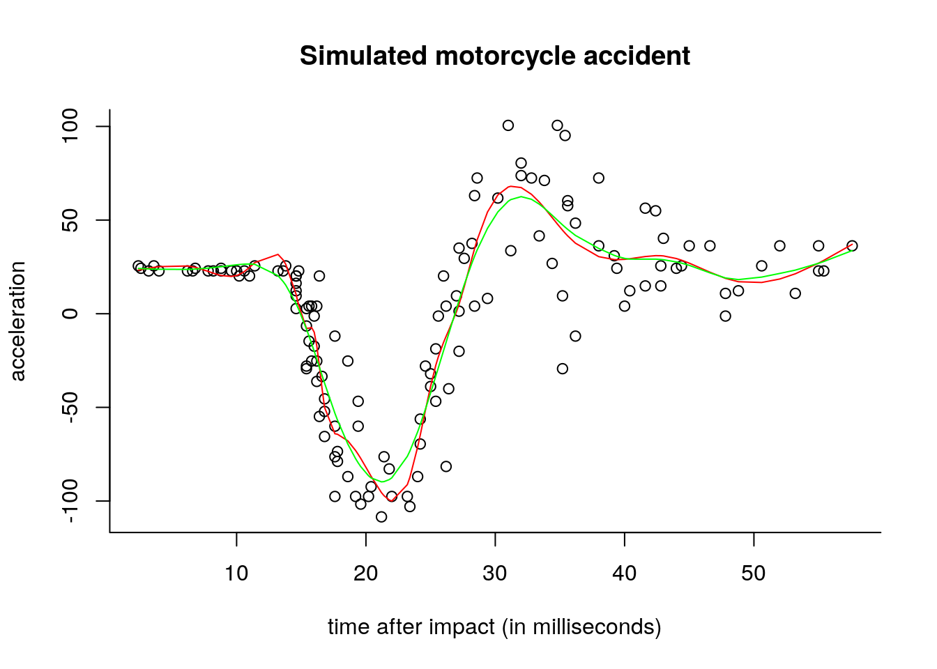
The following illustrates a regression spline in which a number of knots (here roughly \(n/10\)) are chosen equispaced on the distribution scale, based on the quantiles of the covariate vector.
library(splines)
data(mcycle, package = "MASS")
# Center observations
x <- mcycle$times
y <- mcycle$accel - mean(mcycle$accel)
n <- length(x)
df <- floor(n/10)
# Compute number of knots
m <- df + 4
knots <-  quantile(x, prob = (1:m)/(m+1))

#With regression natural cubic spline, equispaced knots on quantile scale
plot(y~x, xlab = "time after impact (in milliseconds)", ylab = "acceleration",
     main = "Simulated motorcycle accident", bty = "l")
lines(x, fitted(lm(y~ns(x = x, knots = knots))), col = "red")
#Smoothing spline, using GCV
spl <- smooth.spline(x = x, y = y, cv = FALSE, all.knots = TRUE)
lines(x, fitted(spl), col = "green")
The fit from the regression spline differs from that of the smoothing spline. The former uses only 18 basis functions and therefore can be fitted using lm, whereas the smoothing spline uses 94 basis functions (this is lower than \(n\) because there are ties in the x vector).
Below is sample code to obtain the \(\mathbf{B}\) and \(\boldsymbol{\Omega}\) matrices, corresponding to the basis functions and the associated penalty.
# You need the fda package installed
# install.packages("fda")
# Function returns B and Omega matrices
smoothsplineb <- function(x){
  require(fda)
  breaks <- sort(unique(x))
  basisfd <- create.bspline.basis(norder = 4, breaks = breaks)
  B <- bsplineS(x, breaks = breaks, norder = 4, nderiv = 0)
  penmat <- bsplinepen(basisfd, Lfd = 2)
  list(basis = B, penmat = penmat)
}

# Compute ridge regression coefficients manually
lmridge <- function(y, X, O = diag(length(y)), lambda){
  as.vector(solve(crossprod(X) + lambda*O, crossprod(X, y)))
}
For the mcycle data, the following lines of code return those matrices.