10.1 Diagnostics for Bernoulli data
This is the example presented in class. The response variable is a binary indicator of low birthweight.
data(birthwt, package = "MASS")
# Preprocessing from MASS - give meaningful labels for factors
# See help for description of the data set
# Rewrite a new data frame with those variables
bwt <- with(birthwt, {
  race <- factor(race, labels = c("white", "black", "other"))
  ptd <- factor(ptl > 0)
  ftv <- factor(ftv)
  # Group number of visits to avoid categories with small counts
  levels(ftv)[-(1:2)] <- "2+"
  data.frame(low = factor(low), age, lwt, race, smoke = (smoke > 0),
             ptd, ht = (ht > 0), ui = (ui > 0), ftv)
  })

lbw <- glm(low ~ ., family = binomial, data = bwt)
# Can use summary just like for lm
summary(lbw)
##
## Call:
## glm(formula = low ~ ., family = binomial, data = bwt)
##
## Deviance Residuals:
## Min 1Q Median 3Q Max
## -1.7038 -0.8068 -0.5008 0.8835 2.2152
##
## Coefficients:
## Estimate Std. Error z value Pr(>|z|)
## (Intercept) 0.82302 1.24471 0.661 0.50848
## age -0.03723 0.03870 -0.962 0.33602
## lwt -0.01565 0.00708 -2.211 0.02705
## raceblack 1.19241 0.53597 2.225 0.02609
## raceother 0.74069 0.46174 1.604 0.10869
## smokeTRUE 0.75553 0.42502 1.778 0.07546
## ptdTRUE 1.34376 0.48062 2.796 0.00518
## htTRUE 1.91317 0.72074 2.654 0.00794
## uiTRUE 0.68019 0.46434 1.465 0.14296
## ftv1 -0.43638 0.47939 -0.910 0.36268
## ftv2+ 0.17901 0.45638 0.392 0.69488
##
## (Dispersion parameter for binomial family taken to be 1)
##
## Null deviance: 234.67 on 188 degrees of freedom
## Residual deviance: 195.48 on 178 degrees of freedom
## AIC: 217.48
##
## Number of Fisher Scoring iterations: 4The summary object returns the coefficients, standard errors and results for the Wald test that \(\beta_i=0\). Note that these will generally differ from the likelihood ratio test.
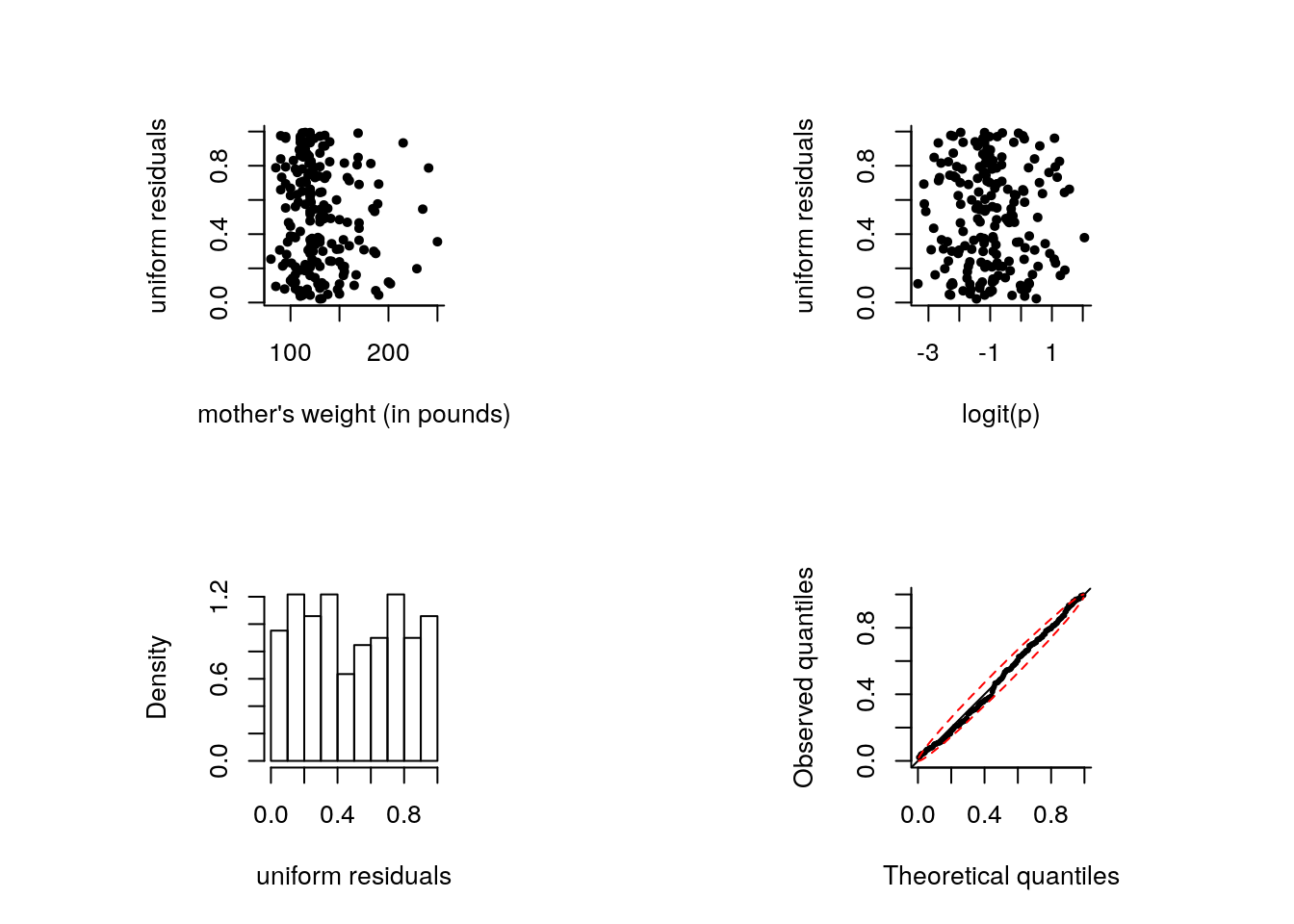
The code above illustrates how to fit the Bernoulli model. Since the data are binary, there is no need to give two columns as response. The following code produces diagnostics for the model as shown in class:
binmod <- glm(formula = low ~ lwt + race + smoke + ptd + ht + ui,
           family = binomial(link = "logit"), data = bwt)
#Logit link function
logit <- function(x){log(x)-log(1-x)}
n <- length(fitted(binmod))
U1 <- runif(n, min = 0, max = fitted(binmod))
U2 <- runif(n, min = fitted(binmod), max = 1)
unires <- binmod$y*U1 + U2*(1-binmod$y)
par(pty = "s", mfrow = c(2, 2), bty = "l", pch = 20)
plot(bwt$lwt, unires, ylab = "uniform residuals",
     xlab = "mother's weight (in pounds)")
plot(logit(fitted(binmod)), unires, ylab = "uniform residuals",
     xlab = "logit(p)")
hist(unires, probability = TRUE, main = "", xlab = "uniform residuals")

# Quantile - quantile plot
plot(x = rank(unires)/(n + 1), y = unires,
     xlab = "Theoretical quantiles", ylab = "Observed quantiles",
     xlim = c(0, 1), ylim = c(0, 1), cex = 0.5)
abline(a = 0, b = 1)
# Simulated confidence bands, based on quantiles of the uniform distribution
pconfint <- apply(apply(matrix(runif(10000 * n), nrow = n), 2, sort), 1, quantile, probs = c(0.025, 0.975))
lines((1:n)/(n+1), pconfint[1,], lty = 2, col = 2)
lines((1:n)/(n+1), pconfint[2,], lty = 2, col = 2)