2.3 The hyperplane of fitted values

In class, we presented a linear model for the Auto dataset of the form \[\mathsf{mpg}_i = \beta_0 + \beta_1 \mathsf{hp}_i + \beta_2 \mathsf{hp}_i^2 + \varepsilon_i\] and claimed this was a linear model. This is indeed true because we can form the design matrix \([\mathbf{1}_n, \mathsf{hp}, \mathsf{hp}^2]\) and obtain coefficients \(\hat{\boldsymbol{\beta}}\). The graphical depiction is counterintuitive.

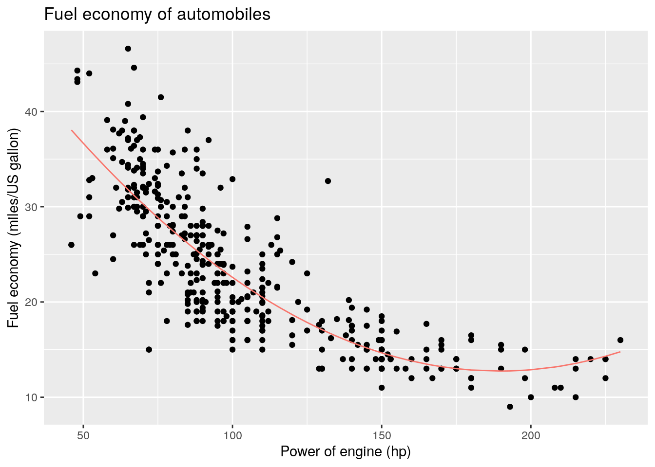
This quadratic curve is nothing like an hyperplane! Let \(\boldsymbol{y} \equiv \texttt{mpg}\), \(\mathsf{x} = \texttt{hp}\) and \(\mathsf{z} = \texttt{hp}^2\). But recall that we are working in three dimensions (the intercept gives the height of the hyperplane) and the coordinates of our hyperplane are
\[\beta_0 + \beta_1x-y +\beta_2z =0.\] However, the observations will always be such that \(z = x^2\), so our fitted values will lie on a one-dimensional subspace of this hyperplane.

The following 3D depiction hopefully captures this better and shows the fitted hyperplane along with the line on which all the (\(x_i, z_i\)) observations lie.