4.5 Solutions
4.5.1 Exercise 7.1 - Study of growth hormones
We will use factor objects in the sequel. A factor encodes a matrix of binary variables,
potentially identied using strings, so that the output is readable. R know how to handle the vector if it is passed to e.g. the function lm. By default, if the matrix spans \(\mathbf{1}_n\), the first level (in alphabetical order) is dropped and the intercept becomes the mean of this level.
url1 <- "https://lbelzile.bitbucket.io/math341/growth.dat"
growth <- read.table(url1, header = TRUE)
summary(growth)
## y x group
## Min. :107.0 Min. : 78.00 control :10
## 1st Qu.:122.0 1st Qu.: 93.75 thiouracil:10
## Median :140.0 Median :100.50
## Mean :142.4 Mean :100.90
## 3rd Qu.:156.5 3rd Qu.:109.25
## Max. :185.0 Max. :123.00##Check what the factor encodes: transpose of design matrix
t(model.matrix(y ~ group - 1, data= growth))## 1 2 3 4 5 6 7 8 9 10 11 12 13 14 15 16 17 18 19 20
## groupcontrol 1 1 1 1 1 1 1 1 1 1 0 0 0 0 0 0 0 0 0 0
## groupthiouracil 0 0 0 0 0 0 0 0 0 0 1 1 1 1 1 1 1 1 1 1
## attr(,"assign")
## [1] 1 1
## attr(,"contrasts")
## attr(,"contrasts")$group
## [1] "contr.treatment"#Fit linear model with interaction
rats_lm <- lm(y ~ x * group, data = growth)
## recall x*group is equivalent to x + group + x:group
## x:group is the interaction term,
## The design matrix can be extracted using the command
model.matrix(rats_lm)## (Intercept) x groupthiouracil x:groupthiouracil
## 1 1 114 0 0
## 2 1 123 0 0
## 3 1 111 0 0
## 4 1 100 0 0
## 5 1 104 0 0
## 6 1 102 0 0
## 7 1 94 0 0
## 8 1 112 0 0
## 9 1 90 0 0
## 10 1 110 0 0
## 11 1 109 1 109
## 12 1 101 1 101
## 13 1 100 1 100
## 14 1 100 1 100
## 15 1 101 1 101
## 16 1 92 1 92
## 17 1 95 1 95
## 18 1 93 1 93
## 19 1 78 1 78
## 20 1 89 1 89
## attr(,"assign")
## [1] 0 1 2 3
## attr(,"contrasts")
## attr(,"contrasts")$group
## [1] "contr.treatment"## 2.5 % 97.5 %
## groupthiouracil -87.550757 134.1308431
## x:groupthiouracil -1.594919 0.60835074.5.2 Exercise 7.2 - Electric production of windmills
The dataset windmill contains measurements of electricity output of wind turbine over 25 separate
fifteen minute periods. We are interested in the relation between direct output and the average wind speed (measured in miles per hour) during
the recording.
- Fit a linear model with wind speed as covariate and plot the standardized residuals against the fitted values. Do you notice any residual structure missed by the model mean specification? Try fitting a model using the reciprocal of wind speed as covariate. Comment on the adequacy of the models.
- Predict, using both models in term, the output of electricity given that the average wind speed in a given period is 5 miles per hour. Provide prediction interval for your estimates.
- Produce a standard Gaussian quantile-quantile plot of the standardized residuals. Superimpose approximate pointwise confidence intervals.
#Extract dataset
url2 <- "https://lbelzile.bitbucket.io/math341/windmill.dat"
windmill <- read.table(file = url2, header = TRUE)
#Copy variables
output <- windmill$output
velocity <- windmill$velocity
recip_velo <- 1/velocity
#Fit linear model
lm_wind1 <- lm(output ~ velocity)
#Summary of fit
summ1 <- summary(lm_wind1)
#Graphical parameters
#mfrow: 1 line 2 column plotting window,
#pch: small dots plotting symbol,
#bty: L console shape)
par(mfrow = c(1, 2), pch = 20, bty = "l")
#Plot and add line of best fit
plot(y = output, x = velocity, xlab = "wind velocity (in mph)")
abline(lm_wind1)
#Repeat with second dataset
summ2 <- summary(lm_wind2 <- lm(output ~ recip_velo))
#alternatively summary(lm_wind2 <- lm(output ~ I(1/velocity)))
#Note above how we can assign variables inside call to other functions
plot(output ~ recip_velo, xlab = "reciprocal wind velocity (in mph)")
abline(lm_wind2)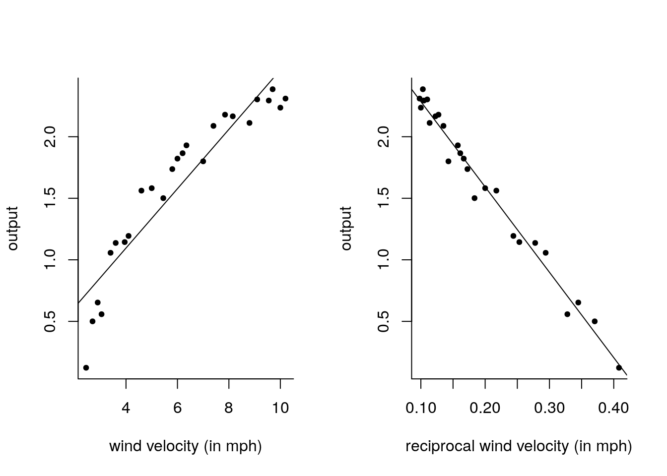
#Standardized residuals r - manual calculation
#Standard deviation of errors
s <- sqrt(sum(resid(lm_wind1)^2)/lm_wind1$df.residual)
#Design matrix i.e. cbind(1, velocity)
Xmat1 <- model.matrix(lm_wind1)
#Dimensions
n <- nrow(Xmat1)
p <- ncol(Xmat1)
#Projection matrix onto Xmat1
Hmat1 <- Xmat1 %*% solve(crossprod(Xmat1)) %*% t(Xmat1)
#Diagonal of H
leverage <- diag(Hmat1)
#Standardized residuals
r_wind1 <- resid(lm_wind1)/(s*sqrt(1-leverage))
#The function rstandard returns those for us
r_wind2 <- rstandard(lm_wind2)

#Plot of standardized residuals vs fitted values
plot(y = r_wind1 - mean(r_wind1), x = fitted(lm_wind1),
     ylab = "Standardized residuals", xlab = "Fitted values",
     main = "Residuals vs\nfitted values", sub ="output ~ velocity")
abline(h = 0, lty = 2)
plot(y = r_wind2 - mean(r_wind2), x = fitted(lm_wind2),
     ylab = "Standardized residuals", xlab = "Fitted values",
     main = "Residuals vs\nfitted values", sub ="output ~ 1/velocity")
abline(h = 0, lty = 2)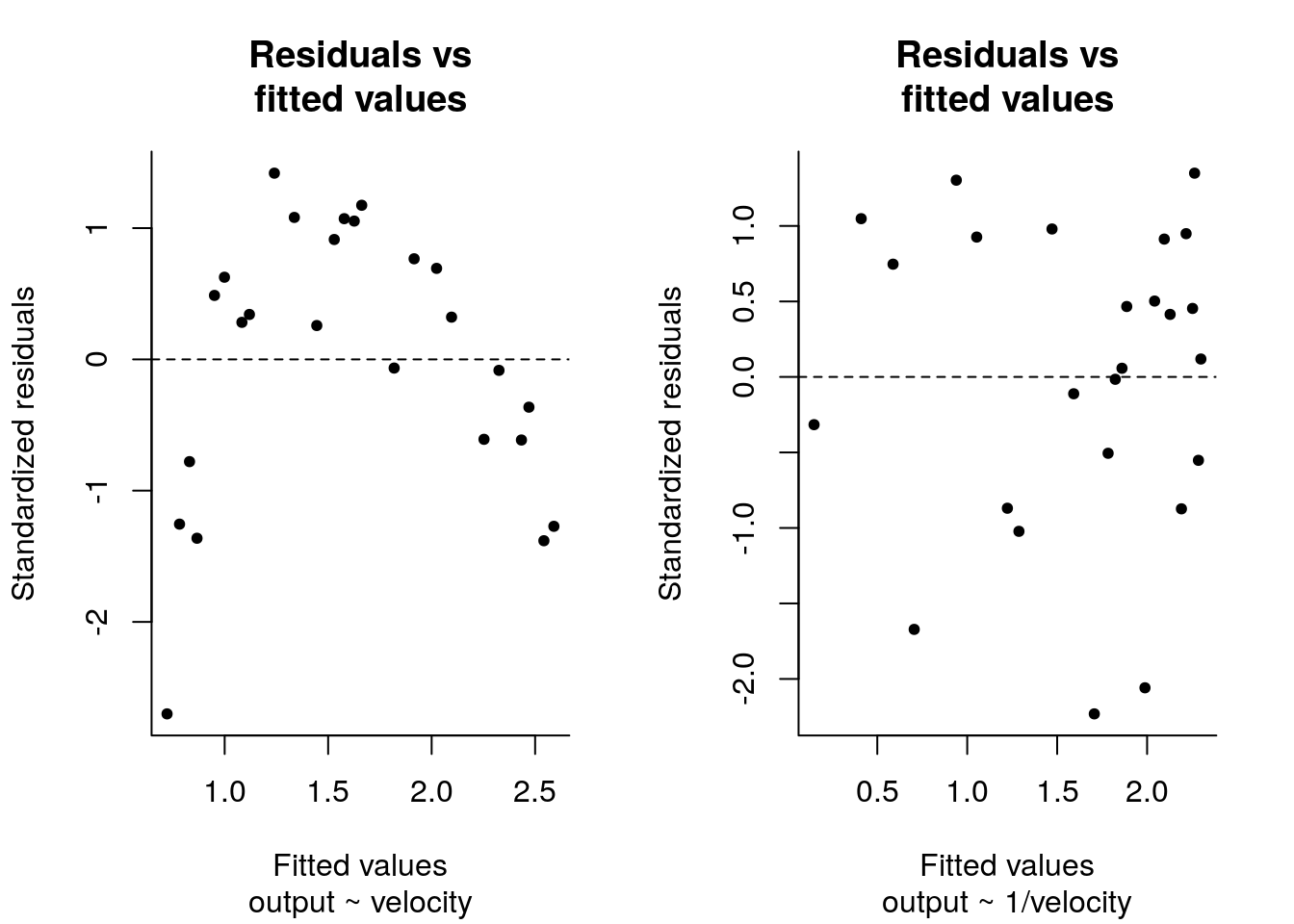
There is some structure left in the model output ~ velocity, since the smallest values occur at the endpoint of the output. There is less visible structure in the model with the reciprocal.
The second model appears to fit better, since its \(\mathrm{R}^2\) value is 0.98 compared to 0.87 for the first model.
Note that, in the second model, the intercept corresponds to infinite strength wind gusts.
#Predict new observation
pred1int <- predict(lm_wind1, newdata = data.frame(velocity = 5),
                    interval = "prediction")
pred2int <- predict(lm_wind2, newdata = data.frame(recip_velo = 1/5),
                    interval = "prediction")
#Manually, see slide 68
xplus <- c(1, 5)
pred1 <- xplus %*% coef(lm_wind1)
interv_length <- qt(0.975, lm_wind1$df.residual) * summ1$sigma *
            sqrt((1 + t(xplus) %*% solve(crossprod(Xmat1)) %*% xplus))
#Check that the calculation is correct
isTRUE(all.equal(c(pred1, pred1 - interv_length, pred1 + interv_length),
                 c(pred1int), check.attributes = FALSE))
## [1] TRUEThe predicted output is 1.34 units of electrity for the first model, while the point forecast is 1.59 for the model with the reciprocal velocity. Both intervals overlap, but the second one [1.39, 1.79] is considerable narrower than the first one, given by [0.84, 1.84].
##
## Call:
## lm(formula = output ~ velocity - 1)
##
## Residuals:
##      Min       1Q   Median       3Q      Max
## -0.51276 -0.17156  0.08675  0.20282  0.36832
##
## Coefficients:
##          Estimate Std. Error t value Pr(>|t|)
## velocity  0.25949    0.00715   36.29   <2e-16 ***
## ---
## Signif. codes:  0 '***' 0.001 '**' 0.01 '*' 0.05 '.' 0.1 ' ' 1
##
## Residual standard error: 0.2364 on 24 degrees of freedom
## Multiple R-squared:  0.9821, Adjusted R-squared:  0.9814
## F-statistic:  1317 on 1 and 24 DF,  p-value: < 2.2e-16
The function update changes the arguments of the linear model. Here, the . means keep all variables on lhs or rhs. You can also use it with a dataset to fit all the remaining variables after specifying the response variable, like for example lm(output ~ ., data = windmill) would have velocity as covariate.
We notice first that the confidence interval for \(\beta_0\), the intercept, includes zero, we cannot reject the null hypothesis that \(\beta_0=0\) at level \(0.95\).
The coefficient \(\beta_1\) corresponding to the effect of velocity has a smaller standard error than the first model. Does this make sense? If a model is correctly specified, addition of new variables that are unrelated does not introduce bias, but ncessarily inflates the standard errors by Gauss–Markov theorem. However, if the intercept should truly be there (this can be made necessary because of measurement errors) and \(\beta_0 \neq 0\), then the tests and confidence intervals will be invalid in the simplified model.
The multiple \(\mathrm{R}^2_c\) goes up the roof, but makes no sense here because it compares two models that are not nested (the model with a single mean versus which has no constant). A consequence of the removal of the intercept is that the average of the residuals is not zero anymore and that R returns different values for the Multiple R-squared.
lm object using -1, the value returned by summary for the coefficient Multiple R-squared is the \(R^2\), not \(R^2_c\)!
We now produce the quantile-quantile plots using the results described in Section 4.4.
Q <- t(qr.Q(qr(Xmat1), complete = TRUE))
resQ1 <- (t(Q) %*% resid(lm_wind1))[-(1:2)]
#Function to add confidence intervals using order statitics
confint.qqplot.ptw <- function(n, dist = "norm", ...){
  t(sapply(1:n, function(i){
  #Beta order statistic quantiles, mapped to scale dist
    do.call(paste0('q', dist), list(qbeta(c(0.025, 0.975), i, n - i + 1), ...))
  }))
}

# Adjust the number of observations
N <- n - p
#Plotting positions on X axis
rankit <- qnorm((1:N) / (N+1))
plot(rankit, sort(scale(resQ1)), xlab = "Theoretical quantiles",
    ylab = "Sample quantiles", main = "Normal Q-Q plot")
abline(a = 0, b = 1)
confint_ptwise <- confint.qqplot.ptw(N)
lines(rankit, confint_ptwise[,1], col = "gray", lty = 2)
lines(rankit, confint_ptwise[,2], col = "gray", lty = 2)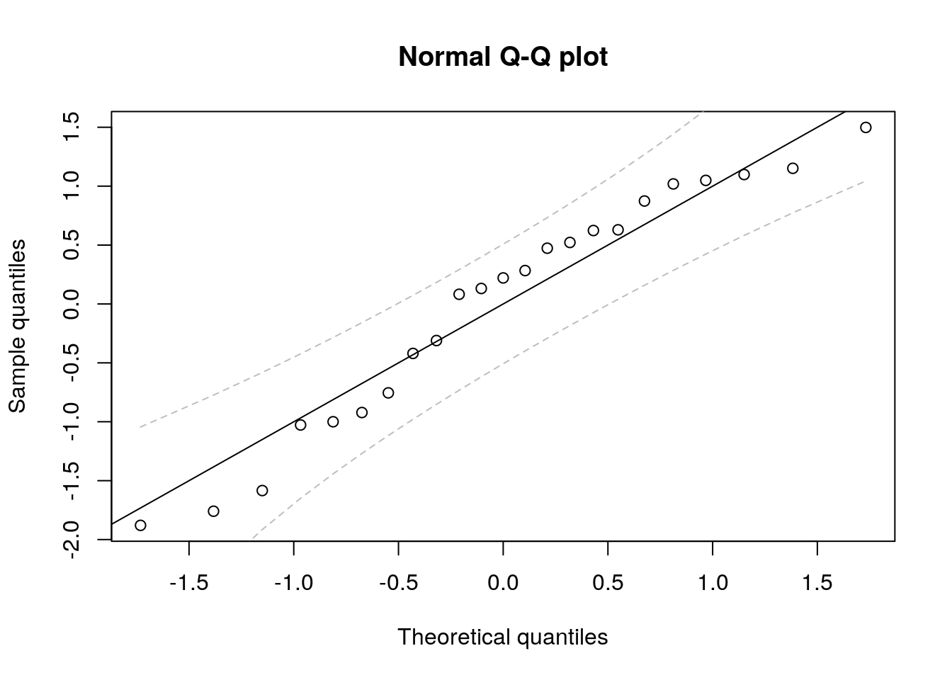
boot_samps <- replicate(sort(scale(rnorm(N))), n = (B <- 9999))
alpha <- 0.05
k <- alpha/2*(B + 1)
confint_boot <- apply(boot_samps, 1, sort)[c(k, B+1-k),]

#Example with second model
Xmat2 <- cbind(1, 1/velocity)
Q <- t(qr.Q(qr(Xmat2), complete = TRUE))
resQ2 <- (t(Q) %*% resid(lm_wind2))[-(1:2)]

plot(rankit, sort(scale(resQ2)), xlab = "Theoretical quantiles",
    ylab = "Sample quantiles", main = "Normal Q-Q plot")
abline(a = 0, b = 1)
confint_ptwise <- confint.qqplot.ptw(N)
#Simulated pointwise bands
lines(rankit, confint_boot[1,], col = "red", lty = 3)
lines(rankit, confint_boot[2,], col = "red", lty = 3)
#Theoretical bands based on order statistics distribution
lines(rankit, confint_ptwise[,1], col = "gray", lty = 2)
lines(rankit, confint_ptwise[,2], col = "gray", lty = 2)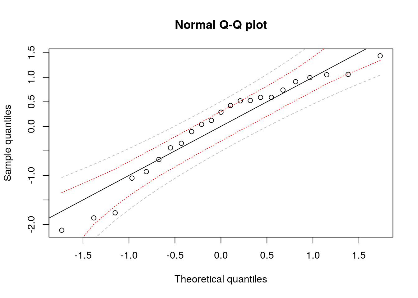
The simulated pointwise confidence interval are shorter and account for the scaling.
4.5.3 Exercise 7.3 - Air traffic
First load the data set and plot the observations
rm(list = ls()) #clear environment
par(bty = "l", pch = 20)
url3 <- "https://lbelzile.bitbucket.io/math341/airpassengers.dat"
airpass <- read.table(file = url3, header = TRUE)
# Cast monthly binary to factor
airpass$time <- airpass$year + (airpass$month-1)/12
airpass$month <- as.factor(airpass$month)
attach(airpass)
#Proceed as usual
plot(y = passengers, x = time, type = "l",
     ylab = "Monthly totals of international airline passengers (in thousands)")
#Fit simple linear model with time as covariate
sum_ap <- summary(fit_ap <- lm(passengers ~ time))
lines(time, fitted(fit_ap), col = 2)
#Create monthly dummies
#create factor using `as.factor
month <- as.factor(rep(1:12, length = length(time)))
levels(month) <- month.abb #abbreviation of months
#A fancier way would convert the fraction to units,
#month <- as.factor(1 + as.integer(c(time*12) %% 12)) # %% is modulo operator
#quarter <- as.factor(rep(1:4, each = 3, length = length(time)))
sum_ad <- summary(fit_ad <- lm(passengers ~ time + month))
lines(time, fitted(fit_ad), lty = 2, col = 4) #dashed blue line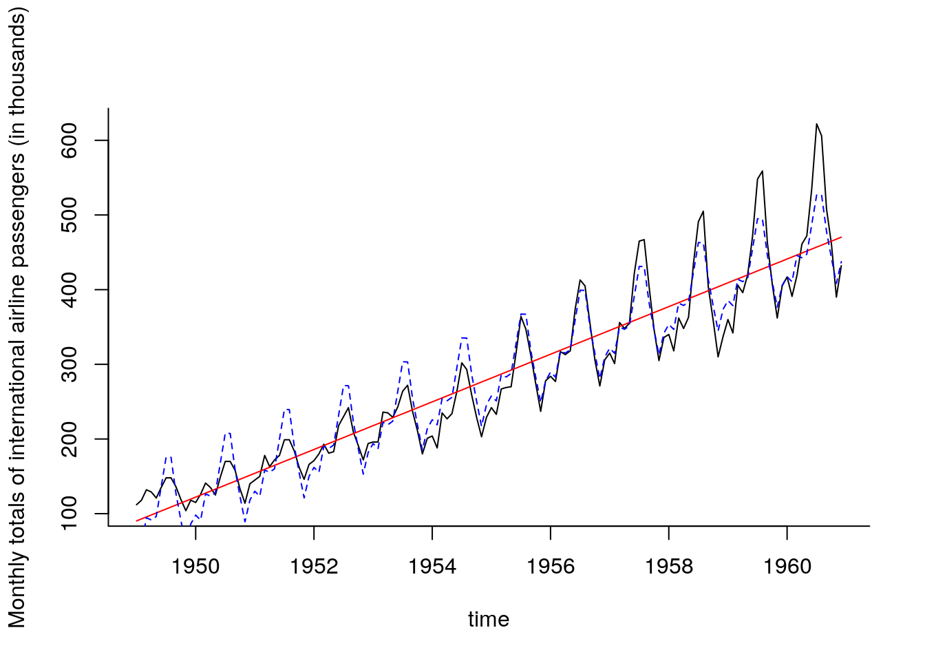
##       1
## 501.263## [,1]
## [1,] 501.263We notice that the model does an overall good job at getting the big features, but misses many things. The first point is that the relationship is not quite linear: a residual plot shows a somewhat quadratic relation between the fitted values and the residuals. The second obvious feature not captured is the change in the variation (the amplitude of the wave pattern changes over time). Since the variance is increasing, a log-transformation may help stabilize it. The residuals are not apparently close to normal (the last values are systematically too large) and there is some skewness. The last few points have large leverage and drive the curve up.
n <- length(passengers)
p <- length(coef(fit_ad))
par(mfrow = c(2, 2))
plot(fit_ad, which = 1) #residuals vs fitted values
plot(fit_ad, which = 2) #Normal Q-Q plot
plot(fit_ad, which = 3) #standardized residuals vs fitted values
plot(fit_ad, which = 4, sub.caption = "") #Cook distance plot
abline(h = 8/(n - 2*p), col = 2)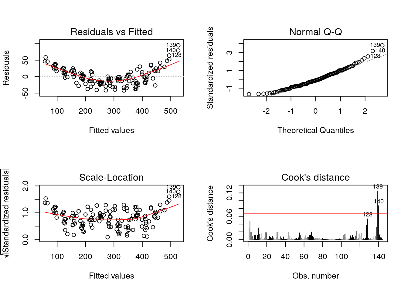
par(mfrow = c(1, 1)) #return to one plot per window
#Compute Cook statistic and other influence statistics
infl_ad <- influence.measures(fit_ad)
cookval_ad <- infl_ad$infmat[,"cook.d"] #cooks.distance
#Diagonal values of the "hat" projection matrix
h_ad <- infl_ad$infmat[, "hat"] #hatvalues
plot(time, rstudent(fit_ad),
     ylab = "Externally studentized residuals",
     xlab = "Time (in years)")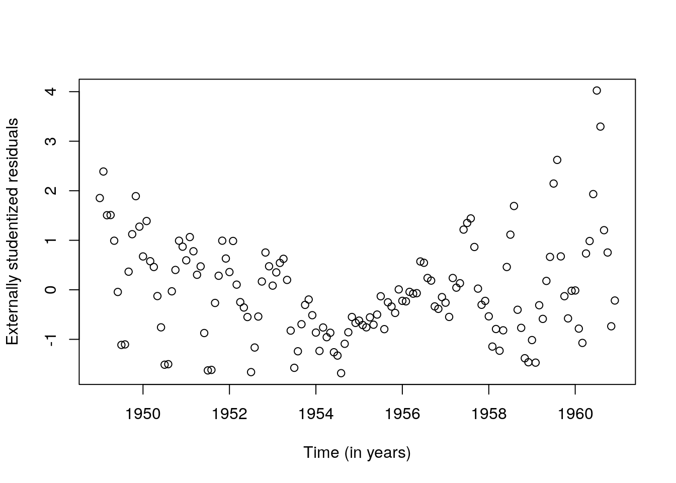
Let us consider the log counts. The fit is much better and the quadratic relationship with the residuals vs fitted values is attenuated. While some points still have high leverage value, they are not considered outliers.
fit_l <- lm(log(passengers) ~ time + month)
plot(log(passengers) ~ time, main = "International airline passengers",
ylab = "log of monthly total count (in thousands)", type = "l")
lines(time, fitted(fit_l), lty = 2, col = 4)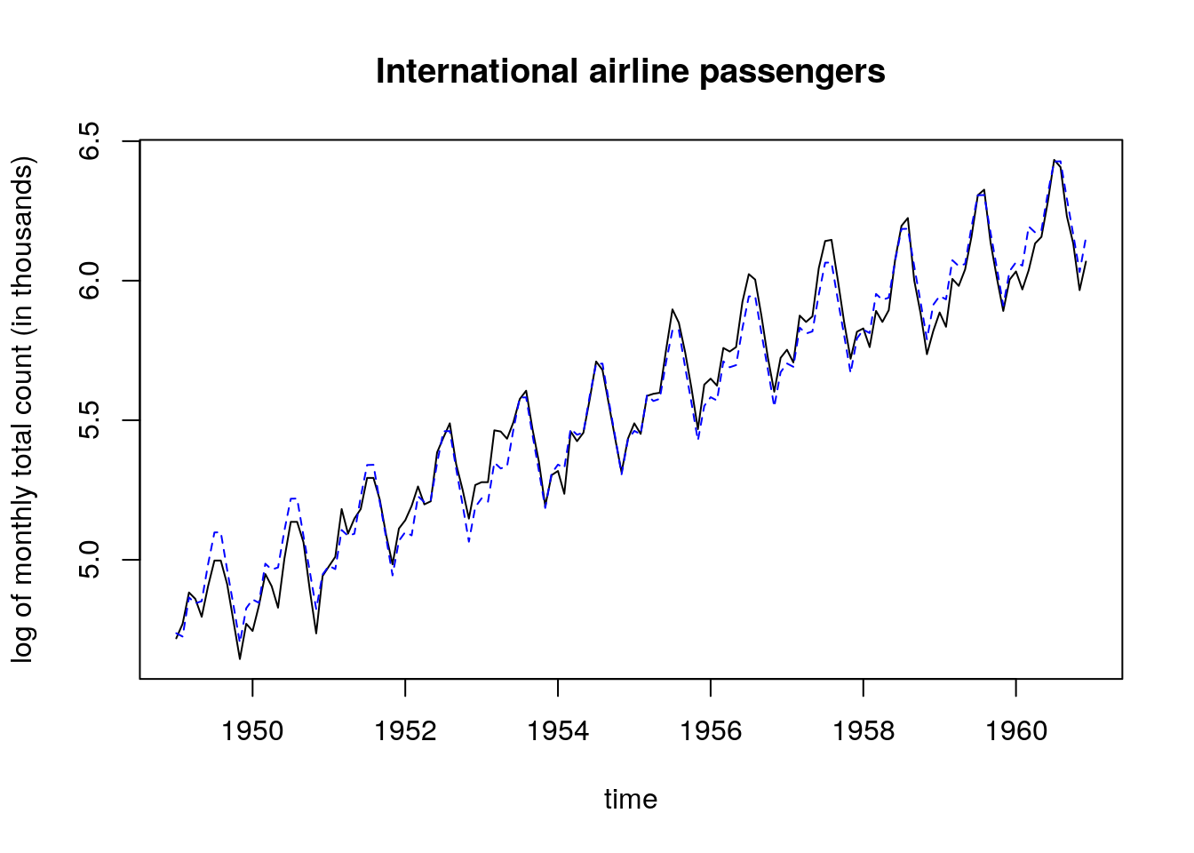
par(mfrow = c(2, 2), pch = 20)
# Q-Q plot
plot(x = qt((1:n)/(n+1), df = n - p + 1), y = sort(scale(rstudent(fit_l))),
     xlab = "Theoretical quantiles", ylab = "Empirical quantiles",
     main = "Quantile-quantile plot of\nexternally studentized residuals")
abline(a = 0, b = 1)
plot(fit_l, which = 1, sub.caption = "")
plot(fit_l, which = 4, sub.caption = "")
abline(h = 8/(n - 2*p), col = 2)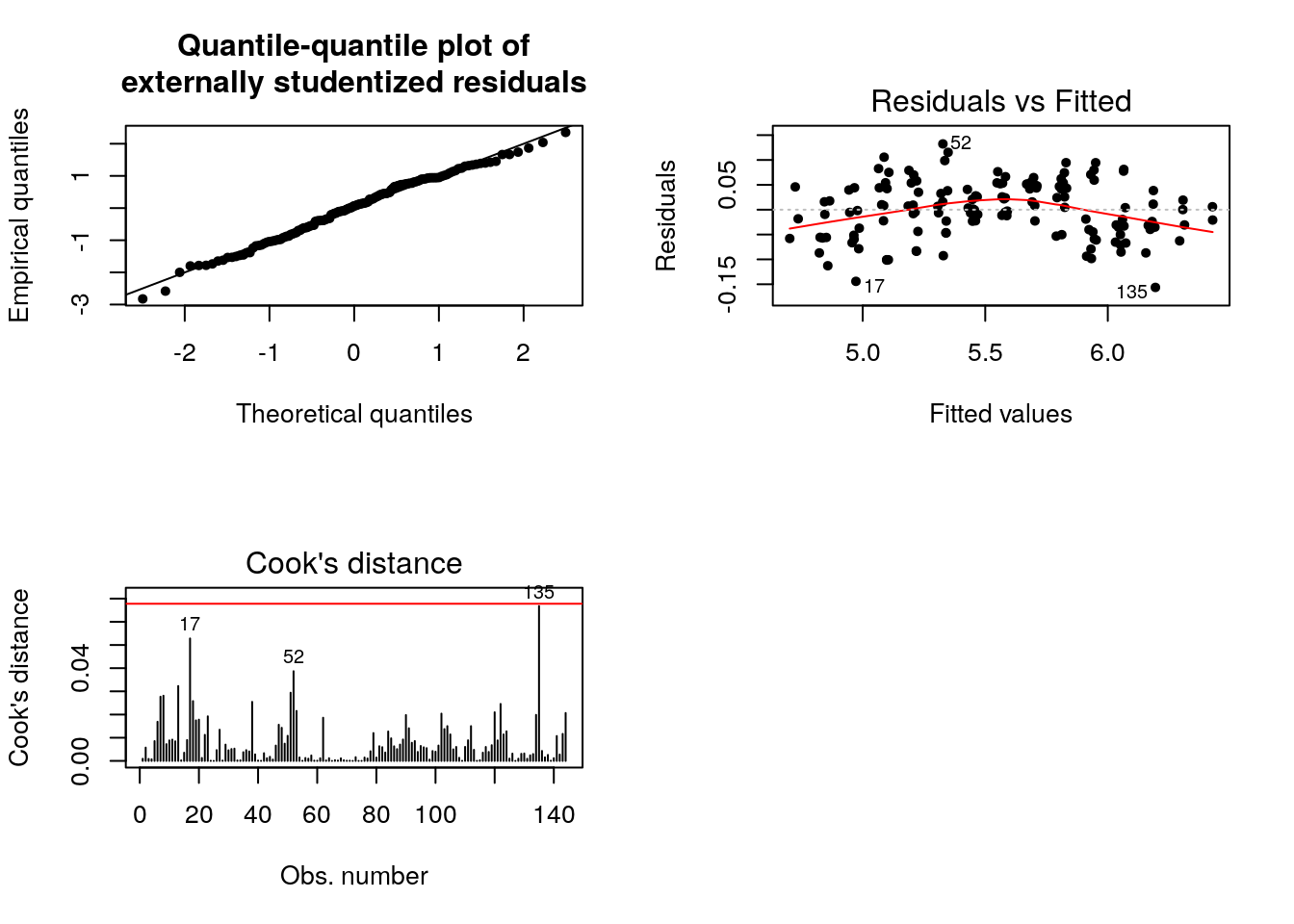
One hypothesis of the linear model that is clearly violated here is the independence of the errors. Even if the variance \(\mathsf{Var}(\boldsymbol{e})=\sigma^2\mathbf{M}_{\mathbf{X}}\) need not have independent errors, there is positive dependence from residual to residual. This is confirmed by looking at the autocorrelation, which indicates geometric decay. This will be covered in MATH 342 (Time Series), but you should just think here of shocks carrying through until the next period before the model reverts to the mean.
Ignoring the serial dependence in the error has consequences: the standard errors are too small (since errors are correlated, there is less units of information so we are overconfident in our uncertainty quantification).
#Laggedresidual plots
par(mfrow = c(1, 1))
plot(x = resid(fit_l)[-1], y = resid(fit_l)[-n],
  ylab = expression(bold(e)[-n]), xlab = expression(bold(e)[-1]),
  main = "Lagged residual plot")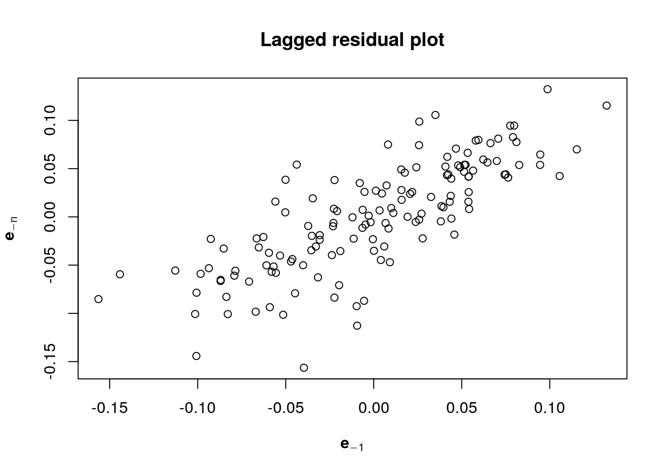
#(partial) correlogram: if residuals have no structure
#there should not be anything outside the bands 19 times out of 20
#Covered in detail in MATH-342 (Time series)
par(mfrow = c(1, 2))
acf(resid(fit_l), main = "Autocorrelation of residuals", xlim = c(1,20))
pacf(resid(fit_l), main = "Partial autocorrelation of residuals")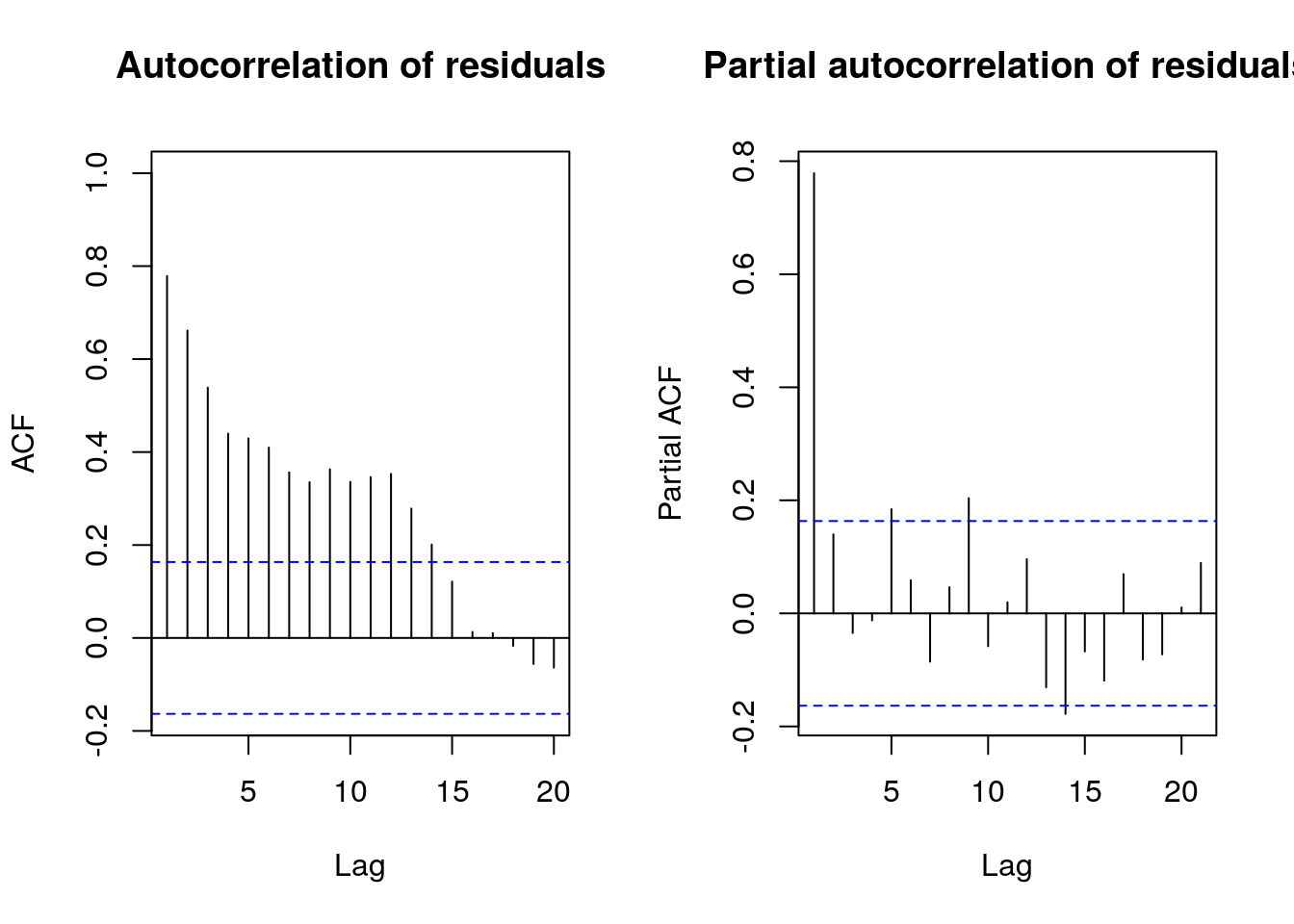
4.5.4 Exercise 7.4 - Determinants of earnings
url4 <- "https://lbelzile.bitbucket.io/math341/labour.dat"
labour <- read.table(url4, header = TRUE, stringsAsFactors = TRUE)
attach(labour)
## Create dummy for extract columns
## additional years of schooling after high school
labour$pseduc  <- I(education >= 13) * (education - 13)
educ_lm <- lm(lhwages ~ education + pseduc, data = labour)
confint(educ_lm)
## 2.5 % 97.5 %
## (Intercept) 2.29267414 2.51468758
## education 0.01030330 0.02940631
## pseduc 0.03325994 0.06318974## Plot with meaningful title + axis label
## red for Male, black for Female
plot(lhwages ~ education, pch = 20, col = as.integer(gender),
bty = "l", ylab = "Log hourly wage (in CAD)",
xlab = "Education achievement (in years)",
main = "Canadian Survey of Labour\nand Income Dynamics (1994)")
## Create observations on a grid, reproducing the design
predic <- cbind(1, 0:20, c(rep(0,12), 1:9)) %*% coef(educ_lm)
lines(0:20, predic, lwd = 2)
## Legend
legend(x = "topleft", legend = c("Man","Woman"),
col = c(2, 1), pch = 20, bty = "n")
## Clear pattern: women are paid less for equivalent qualification

## Add gender as covariate
educ_lm <- lm(lhwages ~ ., data= labour)
# fit lm with all columns but lhwages
## or equivalently
#update(educ_lm, . ~ . + gender)
summary(educ_lm)
##
## Call:
## lm(formula = lhwages ~ ., data = labour)
##
## Residuals:
## Min 1Q Median 3Q Max
## -2.10953 -0.25249 0.02989 0.28176 1.27908
##
## Coefficients:
## Estimate Std. Error t value Pr(>|t|)
## (Intercept) 2.200103 0.055375 39.731 < 2e-16 ***
## education 0.026589 0.004673 5.690 1.38e-08 ***
## genderMale 0.256471 0.014771 17.363 < 2e-16 ***
## pseduc 0.037459 0.007322 5.116 3.31e-07 ***
## ---
## Signif. codes: 0 '***' 0.001 '**' 0.01 '*' 0.05 '.' 0.1 ' ' 1
##
## Residual standard error: 0.4154 on 3183 degrees of freedom
## Multiple R-squared: 0.1897, Adjusted R-squared: 0.1889
## F-statistic: 248.3 on 3 and 3183 DF, p-value: < 2.2e-16## 2.5 % 97.5 %
## (Intercept) 2.09152815 2.30867726
## education 0.01742684 0.03575089
## genderMale 0.22750913 0.28543379
## pseduc 0.02310256 0.05181598The coefficient for gender is still statistically significative at level \(\alpha=5\%\) after adjusting for the education level.