Exercise 12.4 Smoothing splines
# Evaluate GCV at a grid of lambda
lambdas <- seq(0.1, 40, length = 250L)
# Container for GCV criterion
gcv <- rep(0, length(lambdas))
# Loop over cases
for(i in 1:length(lambdas)){
# Compute smoothing matrix
Sm <- B %*% solve(crossprod(B) + lambdas[i]*O) %*% t(B)
# Compute ridge regression coefficients
coefs <- lmridge(y = y, X = B, O = O, lambda = lambdas[i])
# Compute GCV criterion
gcv[i] <- c(crossprod(y - B %*% coefs)/(1-mean(diag(Sm))))/nrow(B)
}
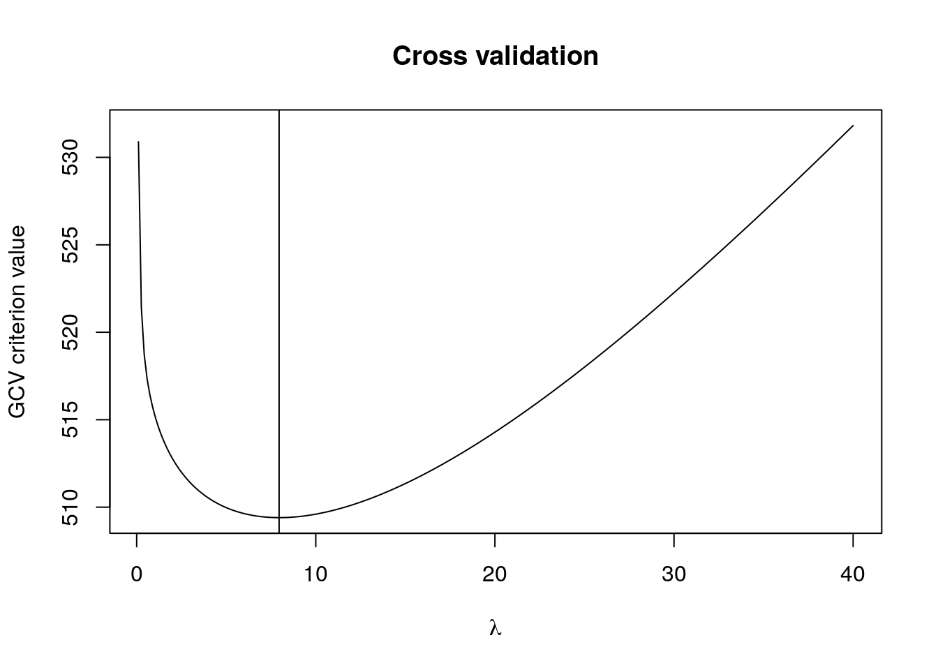
# Plot GCV
plot(lambdas, gcv, type = "l", xlab = expression(lambda),
ylab = "GCV criterion value", main = "Cross validation")
abline(v = lambdas[which.min(gcv)])
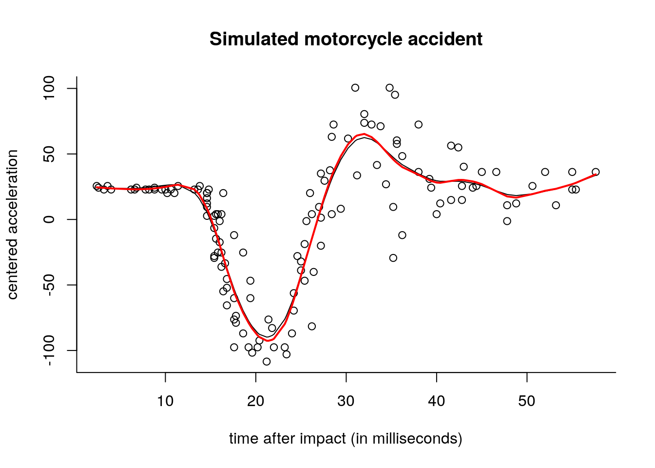
# Plot data
plot(y ~ x, xlab = "time after impact (in milliseconds)", ylab = "centered acceleration",
     main = "Simulated motorcycle accident", bty = "l")
# Undersmoothing
#lines(x, B %*% lmridge(y = y, X = B, O = O, lambda = 0.01), col = "green")
# Oversmoothing
#lines(x, B %*% lmridge(y = y, X = B, O = O, lambda = 500), col = "blue")
lines(predict(smooth.spline(y = y, x = x, all.knots = TRUE)))
fitted_opt <- B %*% lmridge(y = y, X = B, O = O,
                    lambda = lambdas[which.min(gcv)])
lines(x, fitted_opt , col = "red", lwd = 2)