2.4 (Centered) coefficient of determination
Recall the decomposition of observations into fitted and residual vectors, \[\boldsymbol{y} = (\boldsymbol{y} - \mathbf{X}\hat{\boldsymbol{\beta}}) + \mathbf{X}\hat{\boldsymbol{\beta}}= \boldsymbol{e} + \hat{\boldsymbol{y}}\] where \(\boldsymbol{e} \equiv \mathbf{M}_{\mathbf{X}}\boldsymbol{y} \perp \hat{\boldsymbol{y}} \equiv \mathbf{H}_{\mathbf{X}}\boldsymbol{y}\).
The centered coefficient of determination, \(R^2_c\) measures the proportion of variation explained by the centered fitted values relative to the centered observations, i.e., \[ R^2_c = \frac{\|\hat{\boldsymbol{y}}-\bar{y}\mathbf{1}_n\|^2}{\|\boldsymbol{y}-\bar{y}\mathbf{1}_n\|^2}=\frac{\|\hat{\boldsymbol{y}}\|^2-\|\bar{y}\mathbf{1}_n\|^2}{\|\boldsymbol{y}\|^2-\|\bar{y}\mathbf{1}_n\|^2}.\] since the vectors \(\bar{y}\mathbf{1}_n \perp \hat{\boldsymbol{y}}-\bar{y}\mathbf{1}_n\).
Provided that \(\mathbf{1}_n \in \mathscr{S}(\mathbf{X})\), it is obvious that the fitted values \(\hat{\boldsymbol{y}}\) are invariant to linear transformations of the covariates \(\mathbf{X}\) (by which I mean you can transform the design matrix column by column, with \(\mathbf{x}_i \mapsto \alpha_i+\mathbf{x}_i\gamma_i\) for \(i=1, \ldots, p\)). Multiplicative changes in \(\boldsymbol{y}\) lead to an equivalent change in \(\boldsymbol{e}\) and \(\hat{\boldsymbol{y}}\). However, location-changes in \(\boldsymbol{y}\) are only reflected in \(\hat{\boldsymbol{y}}\) (they are absorbed by the intercept). This is why \(R^2\) is not invariant to location-changes in the response, since the ratio \(\|\hat{\boldsymbol{y}}\|^2/\|\boldsymbol{y}\|^2\) increases to 1 if \({\boldsymbol{y}}\mapsto {\boldsymbol{y}}+ a \mathbf{1}_n\).
This invariance is precisely the reason we dismissed \(R^2\). For example, a change of units from Farenheit to Celcius, viz. \(T_c = 5 (T_F - 32)/9\), leads to different values of \(R^2\):
data(aatemp, package = "faraway")
plot(temp ~ year, data = aatemp, ylab = "Temperature (in F)", bty = "l")
#Form design matrix and two response vectors
yF <- aatemp$temp
n <- length(yF)
yC <- 5/9*(aatemp$temp - 32)
X <- cbind(1, aatemp$year)
# Obtain OLS coefficients and fitted values
XtX <- solve(crossprod(X))
beta_hat_F <- XtX %*% crossprod(X, yF)
abline(a = beta_hat_F[1], b = beta_hat_F[2])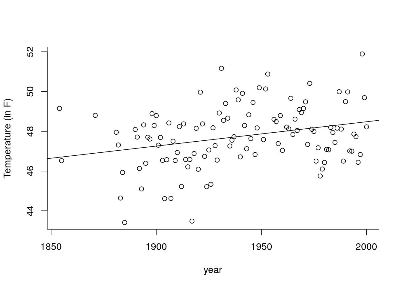
beta_hat_C <- XtX %*% crossprod(X, yC)
fitted_F <- X %*% beta_hat_F
fitted_C <- X %*% beta_hat_C
# Compute coefficient of determination
R2_F <- sum(fitted_F^2)/sum(yF^2)
R2_C <-  sum(fitted_C^2)/sum(yC^2)
#Centered R^2
R2c_F <- sum((fitted_F-mean(yF))^2)/sum((yF-mean(yF))^2)
R2c_C <-  sum((fitted_C-mean(yC))^2)/sum((yC-mean(yC))^2)
isTRUE(all.equal(R2c_F, R2c_C))
## [1] TRUEThe difference \(R^2(F)-R^2(C)=\) 0.00752 is small because the \(R^2\) value is very high, but the coefficient itself is also meaningless. In this example, \(R^2(F)=\) 0.9991, which seems to indicate excellent fit but in fact only 8.54% of the variability is explained by year and we do an equally good job by simply taking \(\hat{y}_i=\bar{y}\).
\(R^2_c\) makes the comparison between the adjusted linear model and the null model with only a constant, which predicts each \(y_i (i=1, \ldots, n)\) by the average \(\bar{y}\).
If \(R^2_c\) gives a very rough overview of how much explanatory power \(\mathbf{X}\) has, it is not a panacea. If we add new covariates in \(\mathbf{X}\), the value of \(R^2_c\) necessarily increases. In the most extreme scenario, we could add a set of \(n-p\) linearly independent vectors to \(\mathbf{X}\) and form a new design matrix \(mX^*\) with those. The fitted values from running a regression with \(\mathbf{X}^*\) will be exactly equal to the observations \(\boldsymbol{y}\) and thus \(R^2_c=1\). However, I hope it is clear that this model will not be useful. Overfitting leads to poor predictive performance; if we get a new set of \(\mathbf{x}_*\), we would predict the unobserved \(y_*\) using its conditional average \(\mathbf{x}_i^*\hat{\boldsymbol{\beta}}\) and this estimate will be rubish if we included too many meaningless covariates.
Other versions of \(R^2_c\) exist that include a penalty term for the number of covariates; these are not widely used and can be negative in extreme cases. We will cover better goodness-of-fit diagnostics later in the course.
lm returns \(R^2_c\) by default (in the summary table, under the label Multiple R-squared. However, if you remove the intercept, you will get \(R^2\) without warning!
Contrast
mod <- lm(mpg ~ horsepower, data = Auto)
rsqc_lm <- summary(mod)$r.squared
#same model, now X = [1 horsepower] and y = mpg
X <- cbind(1, Auto$horsepower)
y <- Auto$mpg
rsq_lm <- summary(lm(y ~ X - 1))$r.squared

#Compute quantities manually
rsqc_man <- c(crossprod(fitted(mod) - mean(y)) / crossprod(y - mean(y)))
isTRUE(all.equal(rsqc_man, rsqc_lm))
## [1] TRUE## [1] TRUE